Summary
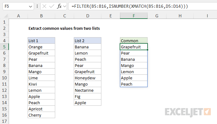
To compare two lists and extract common (i.e. shared) values, you can use a formula based on the FILTER function and the XMATCH function. In the example shown, the formula in F5 is:
=FILTER(B5:B16,ISNUMBER(XMATCH(B5:B16,D5:D14)))
The XMATCH function identifies which values are common to both lists. The FILTER function uses this information to filter the values and return only those that appear in both lists. The seven common values spill into the range F5:F11.
Generic formula
=FILTER(list1,ISNUMBER(XMATCH(list1,list2)))
Explanation
In this example, the goal is to compare the values in two different lists, then extract the values that appear in both lists into a third list as shown in the worksheet above. The values for List 1 appear in column B, and the values for List 2 appear in column D. Although we have a list of fruits in this example, the same approach can be applied to names, places, products, and so on. Also, while the lists in the worksheet are short to make the example easy to understand, the same formula will work fine for lists that contain hundreds or thousands of values.
You can use this same basic approach to extract common values from text strings.
The approach
The general approach for solving this problem is quite simple and looks like this:
- Identify common values in the two lists
- Filter one of the lists to extract common values
The tricky part of the formula is identifying common values. Once we have identified common values, we can extract a list of common values from either list. The generic version of the formula looks like this:
=FILTER(list1,ISNUMBER(XMATCH(list1,list2)))
It does not matter which list we filter, but it is important to provide the same list for the array in FILTER and the lookup_value in XMATCH. This is because we need the resulting array from XMATCH to match the dimensions of the array provided to FILTER. In the worksheet shown, the formula used to solve this problem looks like this:
=FILTER(B5:B16,ISNUMBER(XMATCH(B5:B16,D5:D14)))
At a high level, this formula uses the FILTER function to filter the values in B5:B16 so that only values that appear in both lists are retained. The first step in this process is identifying common values.
Identifying common values
Working from the inside out, the key to this formula is the XMATCH function, which is configured like this:
XMATCH(B5:B16,D5:D14)
Inside XMATCH, the lookup_value is given as the range B5:B16, and the lookup_array is given as D5:D14. Since the lookup item in XMATCH is most often a single value, you might find this configuration strange. Rest assured, there is a method to this madness. In essence, we are asking the XMATCH function to try and find every value in B5:B16 (List 1) in the range D5:D14 (List 2). The result from XMATCH is an array that looks like this:
{#N/A;5;4;1;7;#N/A;#N/A;2;10;3;#N/A;#N/A}
This array is somewhat hard to read, but if you look carefully you will see that it contains 12 items. This makes sense because there are 12 values in the range B5:B16, so each item in the array is a result. The #N/A errors represent values in B5:B16 that were not found in the range D5:D14. The numbers represent the location of values that were found. For example, looking at the first four values in the array:
- The #N/A tells us that "Orange" was not found in D5:D14
- The 5 tells us that "Grapefruit" was found in row 5 of D5:D14
- The 4 tells us that "Pear" was found in row 4 of D5:D14
- The 1 tells us that "Banana" was found in row 1 of D5:D14
And so on. The bottom line is that numbers represent common values that appear in both lists, and errors indicate values in List 1 that were not found in List 2.
XMATCH defaults to an exact match, so match_mode is not required above.
Converting results to TRUE and FALSE
Now that we know which values appear in both lists, the next step is filtering one of the lists to show only common values. However, before we can do that, we need to convert the results from XMATCH into something more digestible to FILTER. If we try to use the array as-is, FILTER will throw an error when it encounters any #N/A error in the array. To do the conversion, we use the ISNUMBER function which is wrapped around XMATCH:
=ISNUMBER(XMATCH(B5:B16,D5:D14))
First, XMATCH returns the array of positions, as described above:
ISNUMBER({#N/A;5;4;1;7;#N/A;#N/A;2;10;3;#N/A;#N/A})
Next, the ISNUMBER function converts these results into simple TRUE and FALSE values. The result is another array like this:
{FALSE;TRUE;TRUE;TRUE;TRUE;FALSE;FALSE;TRUE;TRUE;TRUE;FALSE;FALSE}
Again notice we have 12 items in the array, each corresponding to a value in B5:B16. However, the numbers and errors are gone. In this new array, a TRUE indicates a value that was found, and a FALSE indicates a value that was not found. This is exactly what we need for the FILTER function.
Filtering the values
The final step in the process is to filter the values in B5:B15 by the array we created with XMATCH and ISNUMBER. The result from ISNUMBER is returned directly to FILTER as the include argument with the range B5:B16 given for array:
=FILTER(B5:B16,{FALSE;TRUE;TRUE;TRUE;TRUE;FALSE;FALSE;TRUE;TRUE;TRUE;FALSE;FALSE})
FILTER uses the array to "filter" the values in B5:B16 and only values associated with TRUE survive the operation. The final result from FILTER is an array that contains the seven values common to both lists:
{"Grapefruit";"Pear";"Banana";"Mango";"Lemon";"Apple";"Peach"}
This array lands in cell F5 and spills into the range F5:F11.
Remove duplicates
To remove duplicates, you can nest the formula inside the UNIQUE function:
=UNIQUE(FILTER(list1,ISNUMBER(XMATCH(list1,list2))))
Sort results
To sort results, you can nest the formula inside the SORT function:
=SORT(FILTER(list1,ISNUMBER(XMATCH(list1,list2))))
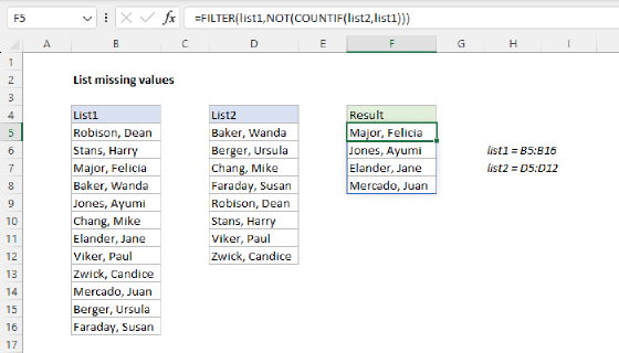
List missing values
To reverse the logic and list values in List 1 that do not appear in List 2 you can modify the formula like this:
=FILTER(list1,ISNA(XMATCH(list1,list2)))
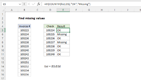
Notice the only change is to replace ISNUMBER with the ISNA function, which returns TRUE for error and FALSE for anything else. For a detailed explanation of this formula, see List missing values.
COUNTIF variation
I want to point out that you can also use the COUNTIF function instead of XMATCH + ISNUMBER to list common values in a formula like this:
=FILTER(B5:B16,COUNTIF(D5:D14,B5:B16))
As before, the array provided to FILTER is the range B5:B16. However, the logic for filtering is done with COUNTIF like this:
COUNTIF(D5:D14,B5:B16)
Here, COUNTIF is configured with D5:D14 as the range and B5:B16 as the criteria. Because we are giving COUNTIF 12 values for criteria, COUNTIF returns 12 results in an array like this:
{0;1;1;1;1;0;0;1;1;1;0;0}
These values are counts. The 1's correspond to values in B5:B16 that also appear in D5:D14 and the zeros correspond to values in B5:B16 that were not found in D5:D14. This array is delivered directly to the FILTER function as the include argument:
=FILTER(B5:B16,{0;1;1;1;1;0;0;1;1;1;0;0})
The FILTER function then filters the values in B5:B16 and returns only those that correspond to a 1. Values associated with 0 are removed. The final result is an array of seven values that exist in both lists, which spills into the range F5:F11.
On the face of it, this is a pretty slick solution that is simpler than the original formula above. However, it comes with a significant caveat: it only works on ranges. This means you cannot create an array of values in a formula and feed it to the COUNTIF variant of this formula, because COUNTIF will not accept an array in place of an actual range. This limitation is shared by all of the IFs functions and is discussed in some detail here. It's frustrating to have a simple and elegant formula that fails in some situations and for this reason, I recommend the XMATCH + ISNUMBER formula as a better, more universal solution.*