Summary
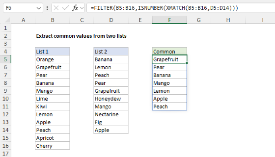
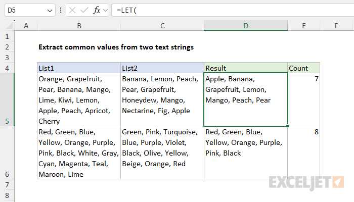
To compare two delimited text strings and extract common values, you can use a formula based on the FILTER function and the XMATCH function with help from the LET function to keep things efficient. In the example shown, the formula in D5 is:
=LET(
list1,TEXTSPLIT(B5,,", "),
list2,TEXTSPLIT(C5,,", "),
common,FILTER(list1,ISNUMBER(XMATCH(list1,list2))),
TEXTJOIN(", ",1,common)
)
As the formula is copied down it returns the values common to both lists. A separate formula in column E returns the count of the common values.
Note: this example builds directly on a more basic example here.
Generic formula
=LET(
list1,TEXTSPLIT(A1,,", "),
list2,TEXTSPLIT(A2,,", "),
common,FILTER(list1,ISNUMBER(XMATCH(list1,list2))),
TEXTJOIN(", ",1,common)
)
Explanation
In this example, the goal is to extract common values from two text strings that contain comma-delimited values. In the worksheet shown the values for "List1" appear in column B and the values for "List2" appear in column C. The results in column D show the intersection of the two lists, that is, the values shared by List1 and List2. Notice that the order of the values in each list is random. In column E, we want to display a count of the common values.
Note: this formula builds directly on another more basic example here, where the values in the lists appear in ranges on the worksheet instead of text strings. I recommend you take a look at that example first since it explains the underlying process in a bit more detail.
The approach
The general approach for solving this problem breaks down into four steps:
- Split the text string for each list into an array of values
- Identify common values in the two arrays
- Filter one of the arrays to extract common values
- Create a comma-separated text string that contains the common values
In addition, I'm using LET in this case to keep the formula efficient and make it easier to read. In the worksheet shown, the formula used to solve this problem looks like this:
=LET(
list1,TEXTSPLIT(B5,,", "),
list2,TEXTSPLIT(C5,,", "),
common,FILTER(list1,ISNUMBER(XMATCH(list1,list2))),
TEXTJOIN(", ",1,common)
)
At a high level, this formula uses the FILTER function to filter the values in list1 to include only values that also appear in list2. The first step in this process is to name some variables.
Splitting the text strings
This formula uses the LET function to define three variables: list1, list2, and common. First, the variable list1 is declared. The value for list1 comes from the TEXTSPLIT function, which is configured to split the text in cell B5 using a comma and a space as a delimiter:
list1,TEXTSPLIT(B5,,", ") // split text in B5 to array
Next, the variable list2 is created in exactly the same way, this time with text from C5:
list2,TEXTSPLIT(C5,,", ") // split text in C5 to array
At this point, list1 is an array that looks like this:
{"Orange";"Grapefruit";"Pear";"Banana";"Mango";"Lime";"Kiwi";"Lemon";"Apple";"Peach";"Apricot";"Cherry"}
And list2 is an array that looks like this:
{"Banana","Lemon","Peach","Pear","Grapefruit","Honeydew","Mango","Nectarine","Fig","Apple"}
Note: Arrays in Excel are very closely related to ranges. You can think of an array as a range of values without an address.
The next step in the formula is to identify common values.
Identifying common values
Working from the inside out, the key to this formula is the XMATCH function, which is configured like this:
XMATCH(list1,list2)
Inside XMATCH, the lookup_value is given as list1, and the lookup_array is given as list2. Since list1 is an array that contains 12 values, XMATCH returns 12 results in an array like this:
{#N/A,5,4,1,7,#N/A,#N/A,2,10,3,#N/A,#N/A}
The #N/A errors represent values in list1 that were not found in list2. The numbers represent the location of values that were found. For example, looking at the first four values in the array:
- The #N/A tells us that "Orange" was not found in list2
- The 5 tells us that "Grapefruit" was found as the fifth value in list2
- The 4 tells us that "Pear" was found as the fourth value in list2
- The 1 tells us that "Banana" was found as the first value in list2
And so on. In other words, the numbers represent values that appear in both lists, and errors indicate values in list1 that were not found in list2.
XMATCH defaults to an exact match, so match_mode is not required above.
Converting results to TRUE and FALSE
Now that we know which values in list1 appear in list2, the next step is to filter list1 to select only common values. However, before we can use FILTER, we need to convert the array returned by XMATCH into TRUE and FALSE values. This is why the XMATCH function is nested inside the ISNUMBER function:
=ISNUMBER(XMATCH(list1,list2))
First, XMATCH returns the array of positions, as described above:
ISNUMBER({#N/A,5,4,1,7,#N/A,#N/A,2,10,3,#N/A,#N/A})
Next, the ISNUMBER function converts these results into simple TRUE and FALSE values. The result is another array like this:
{FALSE,TRUE,TRUE,TRUE,TRUE,FALSE,FALSE,TRUE,TRUE,TRUE,FALSE,FALSE}
Notice we still have 12 items in the array, one for each value in list1. However, the numbers and errors have been replaced by TRUE and FALSE values. A TRUE indicates a value that was found, and a FALSE indicates a value that was not found. This is exactly what we need for the FILTER function.
Filtering the values
The final step in the process is to filter the values in list1 by the array we created with XMATCH and ISNUMBER above. The result from ISNUMBER is delivered to FILTER as the include argument with list1 given for array:
=FILTER(list1,{FALSE,TRUE,TRUE,TRUE,TRUE,FALSE,FALSE,TRUE,TRUE,TRUE,FALSE,FALSE})
FILTER then selects all values in list1 that correspond to TRUE and returns an array that contains the seven values common to both lists:
{"Grapefruit","Pear","Banana","Mango","Lemon","Apple","Peach"}
This array contains just the values shared by list1 and list2. Inside the LET function, we declare a variable named common, and use the array to assign a value:
common,FILTER(list1,ISNUMBER(XMATCH(list1,list2))),
Creating a comma-separated text string
The final step in the process is to join the common values in the comma-separated text string that appears in column D. For this, we use the TEXTJOIN function:
TEXTJOIN(", ",1,common)
With a comma and space (", ") given as a delimiter, TEXTJOIN joins the values in the array returned by FILTER and returns the comma-separated text string in D5 as a final result. When the formula is copied down to D6, the same operation is performed on different text strings that contain colors.
Sort results
To sort results, you can nest the FILTER function inside the SORT function like this:
=LET(
list1,TEXTSPLIT(B5,,", "),
list2,TEXTSPLIT(C5,,", "),
common,SORT(FILTER(list1,ISNUMBER(XMATCH(list1,list2)))),
TEXTJOIN(", ",1,common)
)
Count results
Once you have a list of common values, you can count the values returned in cell D5 with COUNTA and TEXTSPLIT. The formula in cell E5 is:
=COUNTA(TEXTSPLIT(D5,", "))
If you only want a count of common values (not a list), you can calculate the count with an all-in-one formula like this:
=LET(
list1,TEXTSPLIT(B5,,", "),
list2,TEXTSPLIT(C5,,", "),
common,FILTER(list1,ISNUMBER(XMATCH(list1,list2))),
COUNTA(common)
)
This is pretty much the same formula as the original, except for the last line. Instead of joining the values in common with TEXTSPLIT, we count them with COUNTA.
List missing values
To reverse the logic and list values in List 1 that do not appear in List 2 you can modify the formula like this:
=LET(
list1,TEXTSPLIT(B5,,", "),
list2,TEXTSPLIT(C5,,", "),
common,FILTER(list1,ISNA(XMATCH(list1,list2))),
TEXTJOIN(", ",1,common)
)
Notice the only change is to replace ISNUMBER with the ISNA function, which returns TRUE for error and FALSE for anything else.