Find missing values

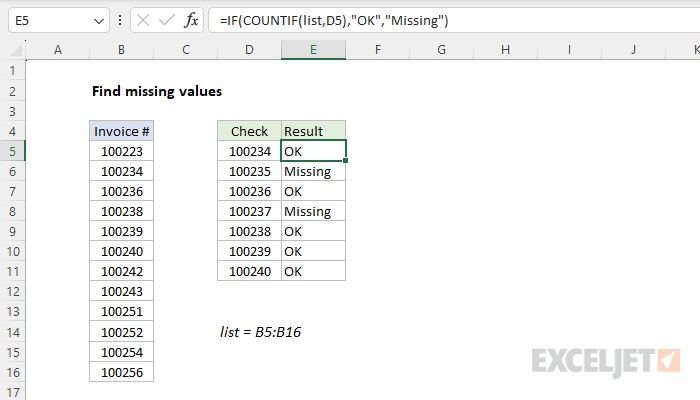
To find values in one list that are missing in another list, you can use a formula based on the COUNTIF function combined with the IF function. In the example shown, the formula in G5 is:

=IF(COUNTIF(list,D5),"OK","Missing")

where list is the named range B5:B16. As the formula is copied down, it returns "OK" when an invoice is found in B5:B16 and "Missing" when an invoice cannot be found.

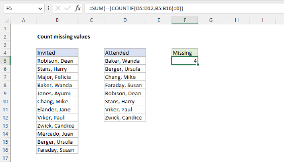
Note: If you want to list missing values, see this page.

Explanation

The goal is to identify invoice numbers in range D5:D11 that are missing in range B5:B16 (named list). Two good ways to solve this problem in Excel are the COUNTIF function and the MATCH function. Both approaches are explained below.

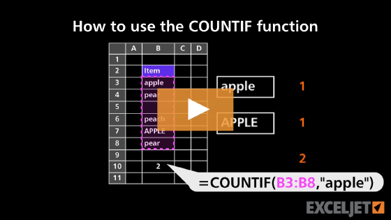
COUNTIF function

COUNTIF counts cells in a range that meet a given condition (criteria). If no cells meet the criteria, COUNTIF returns zero. The generic syntax for COUNTIF is:

=COUNTIF(range,criteria)

To check for missing invoices, combine COUNTIF with the IF function. The formula in G5 is:

=IF(COUNTIF(list,D5),"OK","Missing")

Notice the COUNTIF formula appears inside the IF function as the logical_test argument. Normally, the IF function requires a logical test to return TRUE or FALSE. However, Excel will automatically evaluate any non-zero number as TRUE and the number zero (0) as FALSE. As the formula is copied down column E, COUNTIF returns the count of each invoice in column D in the named range list (B5:B16). When the count is non-zero, The IF function returns "OK". If the invoice is not found in list, COUNTIF returns zero (0), which evaluates as FALSE, and IF returns "Missing".

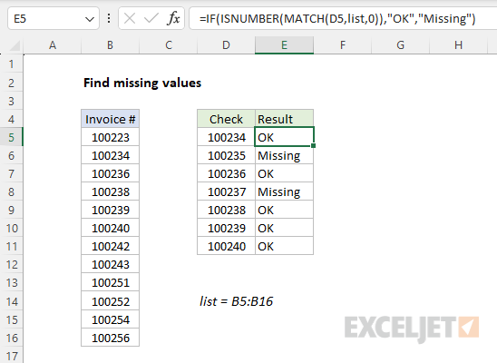
Alternative with MATCH

Another approach is to use the MATCH function. MATCH locates the position of a value in a row, column, or table. The generic syntax for MATCH in exact match mode is:

=MATCH(value,array,0)

The last value, match_type, is set to zero for an exact match. When MATCH finds the lookup value, it returns the position of that value in the array as a number. If MATCH doesn't find the lookup value, it returns an #N/A error. Use this behavior to build a formula that returns "Missing" or "OK" by testing the result of MATCH with the ISNUMBER function:

=IF(ISNUMBER(MATCH(D5,list,0)),"OK","Missing")

As the formula is copied down column E, MATCH returns the position of each invoice in column D in the named range list (B5:B16). When an invoice number is not found, MATCH returns #N/A. The ISNUMBER function returns TRUE or FALSE, depending on the result from MATCH. The result from ISNUMBER is returned to the IF function as the logical_test, and IF then returns "OK" when an invoice is found and "Missing" when an invoice is not found. The screen below shows this formula in use:

Using the MATCH function to find missing values in a column

Summary

The COUNTIF version of this formula and the MATCH version work equally well, but in different ways. Choose based on personal preference. However, one advantage that the MATCH function has over the COUNTIF function is that it will work with in-memory arrays as well as ranges. The COUNTIF function requires a range. This might be important when using dynamic array formulas. To read more about this limitation, see this article.