Summary
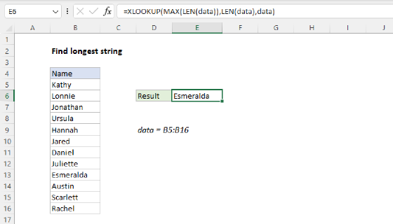
To find the longest string (text value) in a range that meets supplied criteria, you can use the XLOOKUP function together with LEN and MAX. In the example shown, the formula in E6 is:
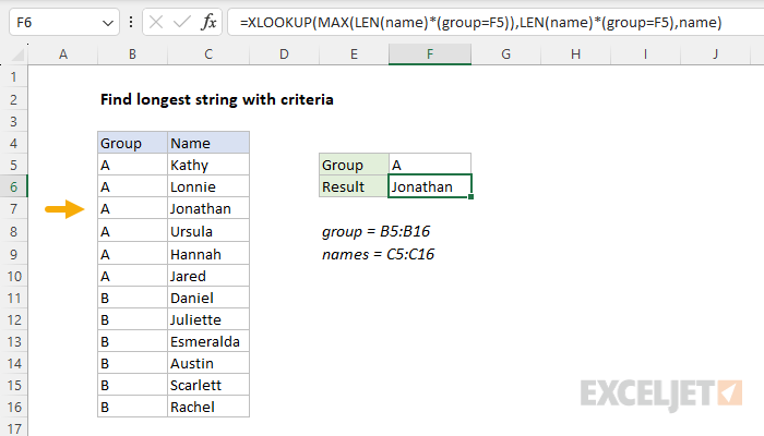
=XLOOKUP(MAX(LEN(name)*(group=F5)),LEN(name)*(group=F5),name)
Where group (B5:B16) and name (C5:C16) are named ranges. The result is "Jonathan", which contains 8 characters and is the longest name in Group A.
Generic formula
=XLOOKUP(MAX(LEN(range)*(criteria)),LEN(range)*(criteria),range)
Explanation
In this example, the goal is to find the longest text string in the range C5:C16 that belongs to the group entered in cell F5. The group is a variable that may be changed at any time. At the core, this is a lookup problem, and the challenge is that the value we need to look up (the string length) does not exist in the data. We need to create this as part of the formula. The easiest way to solve this problem is with the XLOOKUP function. However, in older versions of Excel without the XLOOKUP function, you can use an INDEX and MATCH formula. Both approaches are explained below. For convenience, group (B5:B16) and name (C5:C16) are named ranges, but you can use regular cell references as well.
XLOOKUP solution
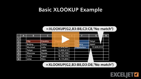
In the workbook shown, the XLOOKUP function returns the longest name in the range C5:C16 when the group value in B5:B16 equals the group entered in cell F5 (which contains "A" in the example shown). The formula in E6 is:
=XLOOKUP(MAX(LEN(name)*(group=F5)),LEN(name)*(group=F5),name)
where group (B5:B16) and name (C5:C16) are named ranges. The result is "Jonathan", which contains 8 characters and is the longest name in group A. The tricky part of this formula is the way we apply the criteria for group, which is done with Boolean algebra. Working from the inside out, we first use the LEN and MAX functions to get the length of the longest name in group A like this:
MAX(LEN(name)*(group=F5))
The LEN function returns the length of a text string in characters. In this case, there are 12 names in data (C5:C16), so LEN returns 12 results in an array like this:
{5;6;8;6;6;5;6;8;9;6;8;6}
We then multiply this array by the expression (group = F5):
=MAX({5;6;8;6;6;5;6;8;9;6;8;6})*(group=F5))
=MAX({5;6;8;6;6;5;0;0;0;0;0;0})
=8
What happens here is that the results from LEN that are not part of group A are "cancelled out" and become zero. The result is returned directly to the MAX function, which returns 8. The result from MAX is delivered to the XLOOKUP function as the lookup_value:
=XLOOKUP(8,LEN(name)*(group=F5),name)
At this point, we have a lookup value of 8, and we need to create a lookup array that holds all string lengths that belong to group A. To do this, we repeat the same process above to create the lookup_array:
=LEN(name)*(group=F5)
={5;6;8;6;6;5;6;8;9;6;8;6}*(group=F5)
={5;6;8;6;6;5;0;0;0;0;0;0}
We can now simplify the formula to this:
=XLOOKUP(8,{5;6;8;6;6;5;0;0;0;0;0;0},name)
XLOOKUP performs an exact match by default. It matches the 8 in the lookup array and returns the corresponding value in name ("Jonathan") as a final result.
INDEX and MATCH solution
In older versions of Excel without the XLOOKUP function, you can use an array formula based on INDEX and MATCH like this:
=INDEX(name,MATCH(MAX(LEN(name)*(group=F5)),LEN(name)*(group=F5),0))
Note: This is an array formula and must be entered with control + shift + enter in Excel 2019 and earlier.