Position of max value in list

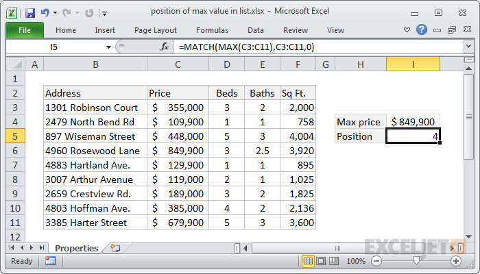
To get the position of the maximum value in a range (i.e. a list, table, or row), you can use the MAX function together with the MATCH function. In the example shown, the formula in I5 is:

=MATCH(MAX(C3:C11),C3:C11,0)

Which returns the number 4, representing the position of the most expensive property in the list.

Explanation

In this formula, the goal is to return the numeric position of the most expensive property in the list. The formula in cell I5 is:

=MATCH(MAX(C3:C11),C3:C11,0)

The MAX function extracts the maximum value from the range C3:C11. In this case, that value is 849900. This number is then supplied to the MATCH function as the lookup value. The lookup_array is the same range (C3:C11), and the match_type is set to "exact" with 0. With those arguments, MATCH finds the maximum value inside the range and returns the relative position of the value in that range.

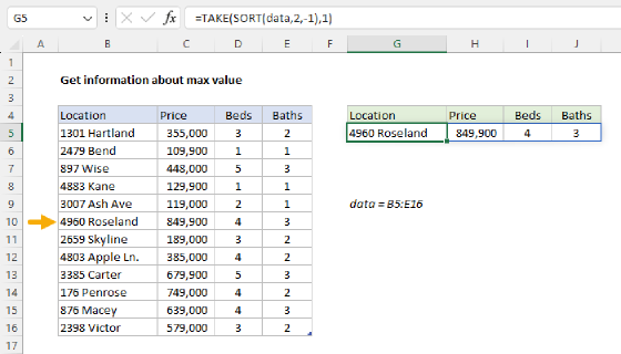
To retrieve information about the most expensive property in the list, we need to add the INDEX function to the mix. See this example for details: Information about the max value.

Notes: (1) In this case, the position corresponds to a relative row number, but in a horizontal range, the position would correspond to a relative column number. (2) In case of duplicates (i.e. two or more max values that are the same) this formula will return the position of the first match, the default behavior of the MATCH function.