Summary
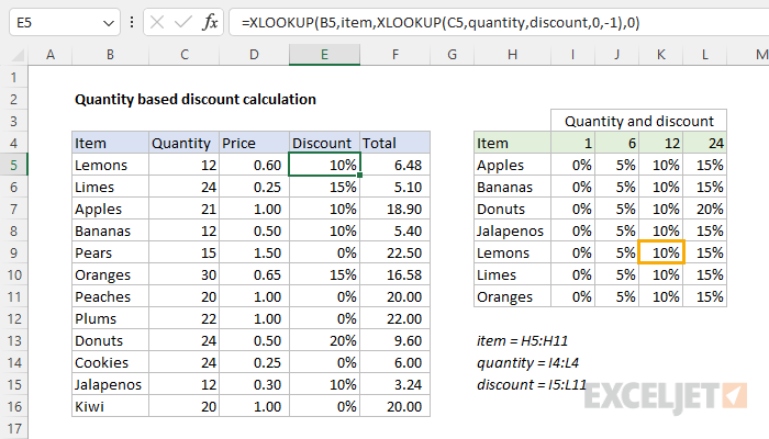
One way to set up a quantity-based discount formula is to place the discounted items in a lookup table, then perform a two-way lookup. In the example shown, the formula in E5 is:
=XLOOKUP(B5,item,XLOOKUP(C5,quantity,discount,0,-1),0)
Where item (H5:H11), quantity (H5:H11), and discount (I5:L11) are named ranges. As the formula is copied down, it references the discount table to determine the correct discount for each item and quantity.
Generic formula
=XLOOKUP(A1,item,XLOOKUP(B1,quantity,discount,0,-1),0)
Explanation
The goal is to calculate discounts on a per-item and per-quantity basis using the discount table at the right in the workbook shown. The purpose of the discount table is to allow each item to have its own set of discounts. Notice that Donuts have a different discount for a quantity of 24. The discounts for other items can be customized as well.
This is a classic two-way lookup problem. The formula must perform an exact match on the item name and an approximate match on the quantity. Note that not all of the items listed in column C appear in the discount table. This means we also need to handle the case of the item not being found (i.e. items that do not appear in the discount table are not discounted). This problem can be solved with XLOOKUP or INDEX and MATCH. Both approaches are explained below.
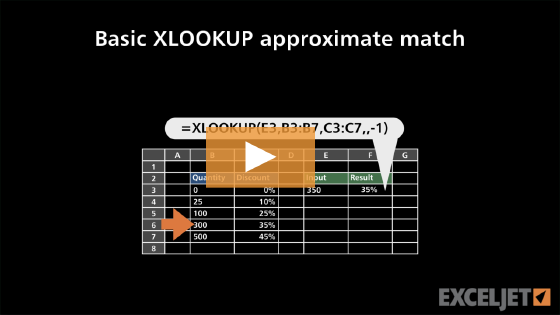
Note: This is a more advanced example. See this page for a very simple quantity-based discount.
Useful links
XLOOKUP solution
One way to solve this problem is with the XLOOKUP function. XLOOKUP is a modern and flexible replacement for older functions like VLOOKUP, and HLOOKUP. The generic syntax for XLOOKUP is:
=XLOOKUP(lookup,lookup_array,return_array,[not_found],[match_mode],[search_mode])
In this problem, the trick is to use XLOOKUP twice: once to retrieve discount information based on the quantity and once to retrieve discount information based on the item. The screen below shows the two lookups that are required:
Let's start with quantity, which is lookup #1 in the screen above. The goal is to retrieve the correct set of discounts for the quantity in column C. To do this, we use XLOOKUP like this:
XLOOKUP(C5,quantity,discount,0,-1)
The lookup_value comes from cell C5. The lookup_array is the named range quantity (I4:L4). For return_array, we provide the named range discount (I5:L11). Because we want a discount of 0% for items that do not appear in the discount table, we provide zero (0) for the if_not_found argument. Finally, because the quantity lookup is not an exact match, we provide -1 for match_mode. This tells XLOOKUP to perform an exact match when available and the next smallest item if not.
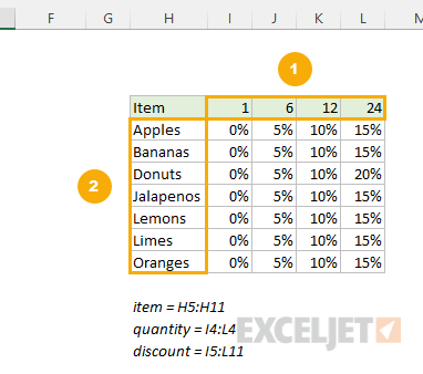
Notice that XLOOKUP will happily accept a horizontal range for lookup_array and that the return_array can be a two-dimensional range containing all discount values. This means that XLOOKUP will return an entire column of discounts after matching a given quantity. For example, with the number 12 in cell C5, XLOOKUP returns all discounts in column K in an array like this:
{0.1;0.1;0.1;0.1;0.1;0.1;0.1}
These decimal values correspond to the percentages seen in the range K5:K11. Because we set match_mode to -1, XLOOKUP will continue to return the same set of discounts until the quantity reaches 24. So, at this point, we have 7 discount values, but we still need to select the correct discount based on the item name. This is lookup #2 in the screen above.
Note: It happens that all discounts for a quantity of 12 are 10%, but the table is structured to allow the discounts to be customized on a per-item basis and the formula will continue to work correctly.
To retrieve the correct discount for an item, we start off like this:
=XLOOKUP(B5,item,
The lookup_value comes from cell B5 and the lookup_array is the named range item (H5:H11). Now we need to add the return_array. This is where things get tricky. If we provide the named range discount, we'll get back all discounts in the matching row. For Lemons, the result looks like this:
=XLOOKUP(B5,item,discount) // returns {0,0.05,0.1,0.15}
However, we don't want all of the discounts for Lemons. Instead, we want the single discount associated with a quantity of 12. So, in order to get that result, we provide lookup formula #1 as the return_array:
=XLOOKUP(B5,item,XLOOKUP(C5,quantity,discount,0,-1)) // returns 0.1
Recall that the result from lookup #1 is the entire column of discounts associated with a quantity of 12. The final result is 0.1 which, when formatted as a percentage, will display as 10%. This is the correct discount for 12 Lemons.
We are nearly finished, but we have one more requirement: when an item is not found in the discount table, we should assume that there is no discount for that item. In other words, we should assume a discount of 0%. To accomplish this in XLOOKUP, we can provide zero for the if_not_found argument. The final formula in cell E5 is:
=XLOOKUP(B5,item,XLOOKUP(C5,quantity,discount,0,-1),0)
As the formula is copied down, it uses the discount table to find the right discount for each item and quantity. When no discount is available for a given item, it returns zero (0).
Applying the discount
The formula in column F calculates the total price for each item and applies the discount in column E with this formula:
=C5*D5*(1-E5) // apply discount
When the discount is zero, the quantity x price calculation is not affected.
INDEX and MATCH option
This problem can also be solved nicely with an INDEX and MATCH formula like this:
=INDEX(discount,MATCH(B5,item,0),MATCH(C5,quantity,1))
This traditional two-way lookup formula is an example of how the INDEX and MATCH can sometimes be more intuitive than using XLOOKUP twice. In a nutshell, we feed the named range discount into the INDEX function as the array argument. For row_num, we use the MATCH function for an exact match on item:
MATCH(B5,item,0) // get row num
For column_num, we use the MATCH function for an approximate match on quantity:
MATCH(C5,quantity,1) // get column num
After the MATCH function is evaluated, we have 5 for row, and 3 for column, and INDEX returns the value at that location:
INDEX(discount,5,3) // returns 0.1
The result is 0.1, which will display as 10% when formatted as a percentage. This is the correct discount for 12 Lemons. Note that if the item is not found in the discount table, MATCH will return #N/A, and INDEX will return the same. To handle the case where the item is not found in the discount table (and therefore the discount should be 0%), we wrap the entire INDEX and MATCH formula inside the IFNA function, and provide zero for value_if_na like this:
=IFNA(INDEX(discount,MATCH(B5,item,0),MATCH(C5,quantity,1)),0)
We could use the IFERROR function instead of IFNA, but IFNA is more specific and therefore a safer option in this case, since it will only trap #N/A errors. For more information about XLOOKUP versus INDEX and MATCH, see this article.
VLOOKUP + MATCH option
Since all discounts are in a single table with the lookup value (Item) in the first column, it is possible to use VLOOKUP + MATCH to solve this problem as well. The trick is to use the MATCH function to locate the right column number to return to VLOOKUP:
=IFNA(VLOOKUP(B5,$H$5:$L$11,MATCH(C5,$H$4:$L$4,1),0),0)
Because VLOOKUP requires the lookup values to be part of the table, and the quantities in row 4 start in the next column, we can't use the named ranges mentioned above directly, so this formula uses absolute references instead. See a more detailed example of a VLOOKUP + MATCH formula here.