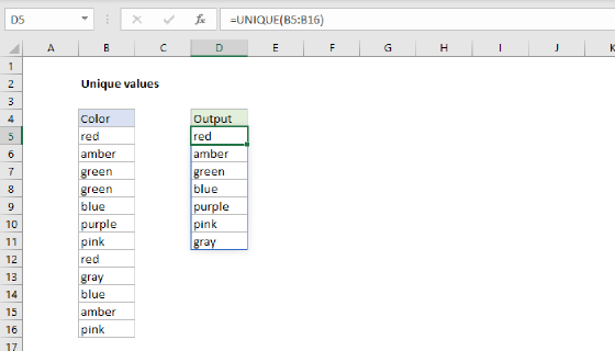
Summary
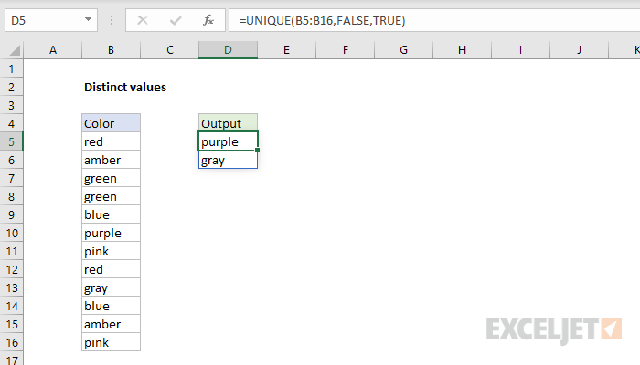
To extract a list of distinct values from a set of data (i.e. values that appear just once), you can use the UNIQUE function. In the example shown, the formula in D5 is:
=UNIQUE(B5:B16,FALSE,TRUE)
which outputs the 2 distinct values in the data, "purple", and "gray".
Generic formula
=UNIQUE(data,FALSE,TRUE)
Explanation
This example uses the UNIQUE function. With default settings, UNIQUE will output a list of unique values, i.e. values that appear one or more times in the source data. However, UNIQUE has an optional third argument, called occurs_once that, when set to TRUE, will cause UNIQUE to return only values that appear once in the data.
In the example shown, UNIQUE's arguments are configured like this:
- array- B5:B16
- by_col - FALSE
- occurs_once - TRUE
Because occurs_once is set to TRUE, UNIQUE outputs the 2 values in the data that appear just once: "purple", and "gray".
Notice the by_col argument is optional and defaults to FALSE, so it can be omitted:
=UNIQUE(data,,TRUE)
TRUE and FALSE can also be replaced with 1 and zero like this:
=UNIQUE(data,0,1)
Dynamic source range
UNIQUE won't automatically change the source range if data is added or deleted. To give UNIQUE a dynamic range that will automatically resize as needed, you can use an Excel Table, or create a dynamic named range with a formula.
UNIQUE is a new function available in Office 365 only.