Summary
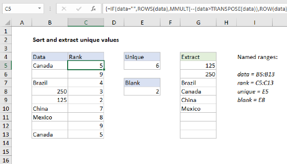
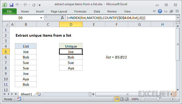
To extract only unique values from a list or column, you can use an array formula based on INDEX and MATCH, and COUNTIF. In the example shown, the formula in D5, copied down, is:
{=INDEX(list,MATCH(0,COUNTIF($D$4:D4,list),0))}
where "list" is the named range B5:B11. This is an array formula and must be entered using control + shift + enter in Excel 2019 and older.
Note: In Excel 365 and Excel 2021, the UNIQUE function provides a better, more elegant way to list unique values and count unique values. These formulas can be adapted to apply logical criteria.
Generic formula
{=INDEX(list,MATCH(0,COUNTIF(uniques,list),0))}
Explanation
The core of this formula is a basic lookup with INDEX:
=INDEX(list,row)
In other words, give INDEX the list and a row number, and INDEX will retrieve a value to add to the unique list.
The hard work is figuring out the ROW number to give INDEX, so that we get unique values only. This is done with MATCH and COUNTIF, and the main trick is here:
COUNTIF($D$4:D4,list)
Here, COUNTIF counts how many times items already in the unique list appear in the master list, using an expanding reference for the range, $D$4:D4.
An expanding reference is absolute on one side, and relative on the other. In this case, as the formula is copied down, the reference will expand to include more rows in the unique list.
Note the reference starts in D4, one row above the first unique entry, in the unique list. This is intentional — we want to count items already in the unique list, and we can't include the current cell without creating a circular reference. So, we start on the row above.
Important: be sure the heading for the unique list does not appear in the master list.
For the criteria in COUNTIF, we are using the master list itself. When given multiple criteria, COUNTIF will return multiple results in an array. At each new row, we have a different array like this:
{0;0;0;0;0;0;0} // row 5
{1;0;0;0;1;0;0} // row 6
{1;1;0;0;1;0;1} // row 7
{1;1;1;1;1;0;1} // row 8
Note: COUNTIF handles multiple criteria with an "OR" relationship (i.e. COUNTIF (range, {"red","blue", "green"}) counts red, blue, or green.
Now we have the arrays we need to find positions (row numbers). For this, we use MATCH, set up for an exact match, to find zero values. If we put the arrays created by COUNTIF above into MATCH, here is what we get:
MATCH(0,{0;0;0;0;0;0;0},0) // 1 (Joe)
MATCH(0,{1;0;0;0;1;0;0},0) // 2 (Bob)
MATCH(0,{1;1;0;0;1;0;1},0) // 3 (Sue)
MATCH(0,{1;1;1;1;1;0;1},0) // 6 (Aya)
MATCH locates items by looking for a count of zero (i.e. looking for items that do not yet appear in the unique list). This works because MATCH always returns the first match when there are duplicates.
Finally, the positions are fed into INDEX as row numbers, and INDEX returns the name at that position.
Non-array version with LOOKUP
You can build a non-array formula to extract unique items using the flexible LOOKUP function:
=LOOKUP(2,1/(COUNTIF($D$4:D4,list)=0),list)
The formula construction is similar to the INDEX MATCH formula above, but LOOKUP can handle the array operation natively.
- COUNTIF returns counts of each value from "list" in the expanding range $D$4:D4
- Comparing to zero creates an array of TRUE and FALSE values
- The number 1 is divided by the array, creating an array of 1s and #DIV/0 errors
- This array becomes the lookup_vector inside LOOKUP
- The lookup value of 2 is larger than any values in the lookup_vector
- LOOKUP will match the last non-error value in the lookup array
- LOOKUP returns the corresponding value in result_vector, the named range "list"
Extract items that appear just once
The LOOKUP formula above is easy to extend with boolean logic. To extract a list of unique items that appear just once in the source data, you can use a formula like this:
=LOOKUP(2,1/((COUNTIF($D$4:D4,list)=0)*(COUNTIF(list,list)=1)),list)
The only addition is the second COUNTIF expression:
COUNTIF(list,list)=1
Here, COUNTIF returns an array of item counts like this:
{2;2;2;2;2;1;2}
which are compared to 1, resulting in an array of TRUE/FALSE values:
{FALSE;FALSE;FALSE;FALSE;FALSE;TRUE;FALSE}
This array acts as a "filter' to restrict output to items that occur just once in the source data.
UNIQUE function in Excel 365
In Excel 365, the UNIQUE function provides a better, more elegant way to list unique values and count unique values. These formulas can be adapted to apply logical criteria.