Filter values in array formula

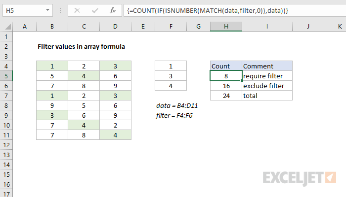
In this example, the goal is to filter the values in one array by the values in another array. For convenience, data (B4:D11) and filter (F4:F6) are named ranges. The solution is based on the MATCH function with the ISNUMBER function. This is a pattern you will see often in more advanced formulas. The formula in cell H5 is:

=COUNT(IF(ISNUMBER(MATCH(data,filter,0)),data))

1. The MATCH function checks all values in the named range data against values in filter
2. ISNUMBER converts matched values to TRUE and non-matched values to FALSE
3. The IF function uses the output in #2 above to perform the actual filtering.

The array returned by the IF function looks like this:

{1,FALSE,3;FALSE,4,FALSE;FALSE,FALSE,FALSE;1,FALSE,3;FALSE,FALSE,FALSE;3,FALSE,FALSE;FALSE,4,FALSE;FALSE,FALSE,4}

As you can see, the values in data that match the values in filter have survived. The values that don't match however have been replaced by FALSE.

The COUNT function is only used to verify the result. Because COUNT automatically ignores the logical values TRUE and FALSE, it returns a count of numbers only, which represent matched values.

Filter to exclude

You can easily reverse the logic to exclude values that appear in filter. In cell H6, the formula has been modified to exclude values using 1-ISNUMBER like so:

=COUNT(IF(1-ISNUMBER(MATCH(data,filter,0)),data))

This effectively reverses the array output in step #2 above.

FILTER function

This example was created before the FILTER function became available. However, the same basic pattern (ISNUMBER + MATCH) works great with FILTER.