Summary
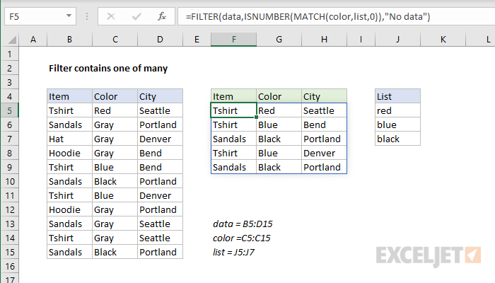
To filter data to include only records where a column is equal to one of many values, you can use the FILTER function together with the ISNUMBER function and MATCH function. In the example shown, the formula in F5 is:
=FILTER(data,ISNUMBER(MATCH(color,list,0)),"No data")
where data (B5:D15), color (C5:C15), and list (J5:J7) are named ranges.
Generic formula
=FILTER(data,ISNUMBER(MATCH(rng1,rng2,0)),"No data")
Explanation
The FILTER function can filter data using a logical expression provided as the include argument. In this example, this argument is created with an expression that uses the ISNUMBER and MATCH functions like this:
=ISNUMBER(MATCH(color,list,0))
MATCH is configured to look for each color in C5:C15 inside the smaller range J5:J7. The MATCH function returns an array like this:
{1;#N/A;#N/A;#N/A;2;3;2;#N/A;#N/A;#N/A;3}
Notice numbers correspond to the position of "found" colors (either "red", "blue", or "black"), and errors correspond to rows where a target color was not found. To force a result of TRUE or FALSE, this array goes into the ISNUMBER function, which returns:
{TRUE;FALSE;FALSE;FALSE;TRUE;TRUE;TRUE;FALSE;FALSE;FALSE;TRUE}
The array above is delivered to the FILTER function as the include argument, and FILTER returns only rows that correspond to a TRUE value.
With hardcoded values
The example above is created with cell references, where target colors are entered in the range J5:J7. However, by using an array constant, you can hardcode values into the formula like this with the same result:
=FILTER(data,ISNUMBER(MATCH(color,{"red","blue","black"},0)),"No data")
Dynamic Array Formulas are available in Office 365 only.