Summary
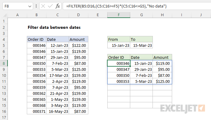
To filter data to extract records between two dates, you can use the FILTER function with Boolean logic. In the example shown, the formula in F8 is:
=FILTER(B5:D16,(C5:C16>=F5)*(C5:C16<=G5),"No data")
The result is a list of records with dates between 15-Jan-23 and 15-Mar-23, inclusive.
Generic formula
=FILTER(data,(dates>=A1)*(dates<=A2),"No data")
Explanation
The goal is to extract records with dates that are greater than or equal to a start date in F5 and less than or equal to an end date in G5. You might think we can use the AND function inside FILTER to solve this problem. However, because AND returns just a single value, this won't work. Instead, we use something called "Boolean logic" to validate the dates.
Background study
Use the links below to learn the concepts explained in this article.
- How to use the FILTER function - overview with examples
- FILTER function basic example - 3 min intro video
- Boolean logic in Excel - 3 min video
- Boolean operations in array operations - 3 min video
- Dynamic array formulas - paid training
FILTER function
This formula uses the FILTER function to retrieve data based on a logical test created with a Boolean logic expression. The array argument is provided as B5:D16, which contains the full set of data without headers. The include argument is based on two logical comparisons:
(C5:C16>=F5)*(C5:C16<=G5)
This is an example of Boolean logic. The expression on the left checks if dates are greater than or equal to the "From" date in F5. The expression on the right checks if dates are less than or equal to the "To" date in G5. The two expressions are joined with a multiplication operator (*), which creates an AND relationship. After logical expressions are evaluated, we have two arrays that contain TRUE and FALSE values like this:
{FALSE;TRUE;TRUE;TRUE;TRUE;TRUE;TRUE;TRUE;TRUE;TRUE;TRUE;TRUE}*{TRUE;TRUE;TRUE;TRUE;TRUE;FALSE;FALSE;FALSE;FALSE;FALSE;FALSE;FALSE}
Notice there are 12 results in each array, one for each date in the data. The multiplication operation automatically converts the TRUE and FALSE values to 1s and 0s, so you should visualize the operation like this:
{0;1;1;1;1;1;1;1;1;1;1;1}*{1;1;1;1;1;0;0;0;0;0;0;0}
After multiplication is complete, the final result is a single array like this:
{0;1;1;1;1;0;0;0;0;0;0;0}
Note that there are four 1s in the array, which correspond to the four dates that pass the logical test. This array is delivered to the FILTER function as the include argument and used to filter the data:
=FILTER(B5:D16,{0;1;1;1;1;0;0;0;0;0;0;0},"No data")
Only the rows with a result of 1 are included in the final output. The if_empty argument is set to "No data" in case no matching data is found.
For more details on FILTER, see: How to use the FILTER function.
With hardcoded start and end dates
In the example shown, we are picking up valid dates from cells F5 and G5. This makes the formula easier to write and more flexible since the dates can easily be changed at any time. However, in certain situations, you may want to hardcode dates into the formula. The safest way to do this in Excel is to use the DATE function as shown below:
=FILTER(B5:D16,(C5:C16>=DATE(2023,1,15))*(C5:C16<=DATE(2023,3,15)),"No data")
The structure of this formula is the same as the original formula above, but the start date of January 15, 2023, and the end date of March 15, 2023, are now provided directly with the DATE function.