Explanation
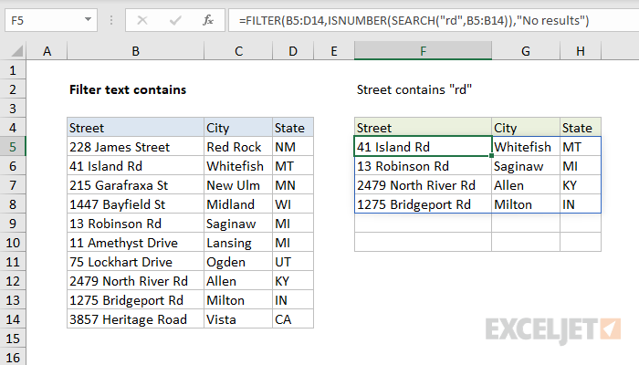
This formula relies on the FILTER function to retrieve data based on a logical test. The array argument is provided as B5:D14, which contains the full set of data without headers. The include argument is based on a logical test based on the ISNUMBER and SEARCH functions:
ISNUMBER(SEARCH("rd",B5:B14))
In brief, the SEARCH function is set up to look for the text "rd" inside the street data in B5:B14. Because this range includes 10 cells, 10 results are returned. Each result is either a number (text found) or a #VALUE error (text not found):
{#VALUE!;11;#VALUE!;#VALUE!;13;#VALUE!;#VALUE!;18;17;#VALUE!}
This array is delivered to the ISNUMBER function, which converts the result from SEARCH into an array that contains only TRUE or FALSE:
{FALSE;TRUE;FALSE;FALSE;TRUE;FALSE;FALSE;TRUE;TRUE;FALSE}
The array from ISNUMBER is provided to the FILTER function as the include argument, and FILTER uses this array to retrieve matching data. Only rows where the result is TRUE make it into the final output. The if_empty argument is set to "No results" in case no matching data is found.
Wildcards
The SEARCH function supports wildcards, so the filter logic can include these characters.
Case-sensitive
For a partial match, case-sensitive filter, you can adjust the formula to use the FIND function instead of SEARCH like this:
=FILTER(rng1,ISNUMBER(FIND("TXT",rng2)))
Note: FIND is case-sensitive, but does not support wildcards.


