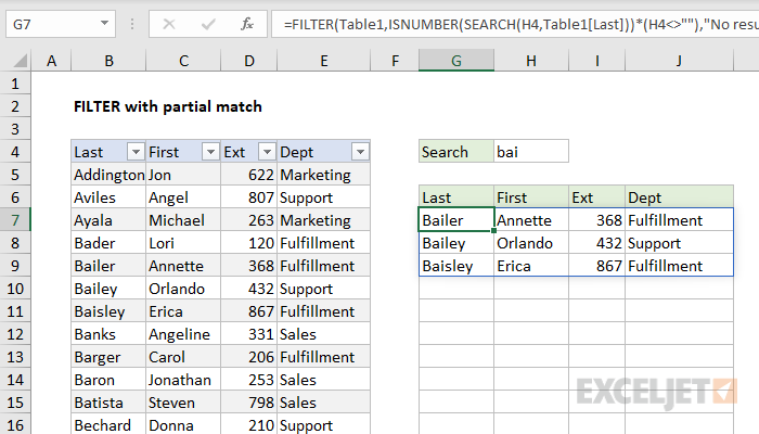
Explanation
In this example, the goal is to extract a set of records that match a partial text string. To keep things simple, we are only matching one field in the data, the last name ("Last"). The core operation of this formula comes from the FILTER function (new in Excel 365) which extracts matching data from a range based on a logical filter:
=FILTER(data,logic)
The challenge in this example is to construct the logic needed to match records based on a partial match. The FILTER function does not support wildcards, so we need to use a different approach. In this case, we are using the SEARCH function together with the ISNUMBER function like this:
ISNUMBER(SEARCH(H4,Table1[Last])) // partial match logic
Here, the SEARCH function is configured to look for text entered in cell H4, inside the "Last" column in the table. If SEARCH finds a result, it returns the position of that result in the text. For example:
=SEARCH("cat","The cat in the hat") // returns 5
If SEARCH doesn't find anything, it returns the #VALUE! error:
=SEARCH("dog","The cat in the hat") // returns #VALUE!
In other words, if SEARCH returns a number, we have a match. If not, we don't have a match. To convert this result into a simple TRUE/FALSE value, we wrap the SEARCH function inside the ISNUMBER function. ISNUMBER will return TRUE only when SEARCH has returned a number:
=ISNUMBER(SEARCH("cat","The cat in the hat")) // returns TRUE
=ISNUMBER(SEARCH("dog","The cat in the hat")) // returns FALSE
Notice we are not using a wildcard like ("*") to get a partial match, but the SEARCH + ISNUMBER combo behaves like a partial match nonetheless. If the search string is found anywhere in the text, SEARCH will return a number and ISNUMBER will return TRUE.
Getting back to the example shown, we are using SEARCH and ISNUMBER like this:
ISNUMBER(SEARCH(H4,Table1[Last])) // partial match logic
Because the table contains 100 rows, the snippet above will generate 100 TRUE/FALSE results, one for each cell in the Last column. This is exactly what we need for the FILTER function – a TRUE or FALSE value for each row in the data. When the snippet above is embedded in FILTER as the include argument, FILTER returns the matching rows:
=FILTER(Table1,ISNUMBER(SEARCH(H4,Table1[Last]))
We now have a working formula but need to tidy up a few things. First, if the FILTER function does not return any match, it will return a #CALC! error. To provide a more friendly message, we add a text message for the if_empty argument:
=FILTER(Table1,ISNUMBER(SEARCH(H4,Table1[Last])),"No results")
Now if the search text isn't found, FILTER will return "No results".
Finally, we need to handle the case of the search text in H4 being empty. Somewhat oddly, the SEARCH function will return the number 1 if the search text is an empty string:
=ISNUMBER(SEARCH("","The cat in the hat")) // returns 1
This will cause FILTER to return all results if cell H4 is empty, since ISNUMBER will happily return TRUE for number 1. To prevent this behavior, we tack on a bit of logic to the original logical expression:
ISNUMBER(SEARCH(H4,Table1[Last]))*(H4<>"")
The expression H4<>"" returns TRUE only when H4 is not empty, and FALSE when H4 is empty. When we multiply the results of this expression by the original SEARCH + ISNUMBER expression, it will "cancel out" all TRUE results when H4 is empty. This is a form of Boolean logic. The math operation of multiplication (*) works like AND logic in array formulas.
Partial match with INDEX and MATCH
The FILTER function is available only in Excel 365. In older versions of Excel, it is possible to set up a partial match formula to return more than one match, but it is more complicated. This formula shows one approach based on INDEX and MATCH.


