Summary
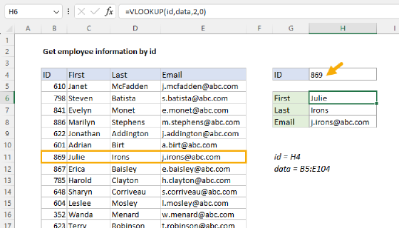
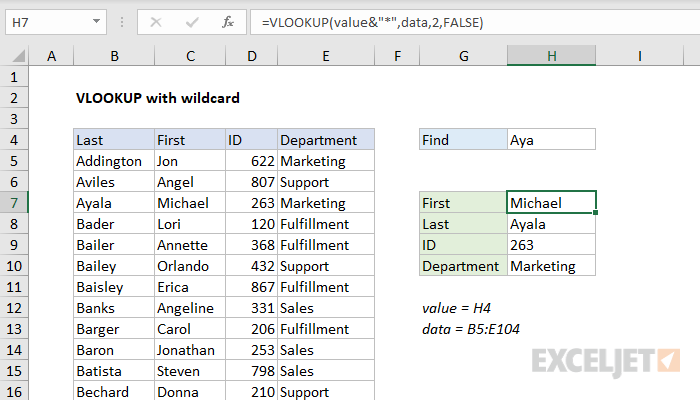
To retrieve information from a table based on a partial match, you can use the VLOOKUP function in exact match mode with a wildcard. In the example shown, the formula in H7 is:
=VLOOKUP(value&"*",data,2,FALSE)
where value (H4) and data (B5:E104) are named ranges.
Generic formula
=VLOOKUP(value&"*",data,column,FALSE)
Explanation
In this example, the goal is to retrieve employee information from a table using only a partial match on the last name. In other words, by typing "Aya" into cell H4, the formula should retrieve information about Michael Ayala.
The VLOOKUP function supports wildcards, which makes it possible to perform a partial match on a lookup value. For instance, you can use VLOOKUP to retrieve values from a table based on typing in only part of a lookup value. To use wildcards with VLOOKUP, you must specify exact match mode by providing FALSE or 0 (zero) for the last argument called range_lookup.
In this example, we use the asterisk (*) as a wildcard which matches zero or more characters. To allow a partial match of the value typed into H4, which is named "value," we supply a lookup value to VLOOKUP like this:
value&"*" // create lookup value
This expression joins the text in the named range value with a wildcard using the ampersand (&) to concatenate. If we type a string like "Aya" into the named range value (H4), the result is "Aya*", which is returned directly to VLOOKUP as the lookup value. Placing the wildcard at the end results in a "begins with" match. This will cause VLOOKUP to match the first entry in column B that begins with "Aya."
Wildcard matching is convenient because you don't have to type in a full name, but you must be careful of duplicates or near duplicates. For example, the table contains both "Bailer" and a "Bailey," so typing "Bai" into H4 will return only the first match ("Bailer"), even though there are two names that begin with "Bai."
Note: in Excel 365, the FILTER function can display all matches at the same time.
Other columns
The formulas in the range H7:H10 are very similar; the only difference is the column index:
=VLOOKUP(value&"*",data,2,FALSE) // first
=VLOOKUP(value&"*",data,1,FALSE) // last
=VLOOKUP(value&"*",data,3,FALSE) // id
=VLOOKUP(value&"*",data,4,FALSE) // dept
Contains type match
For a "contains type" match, where the search string can appear anywhere in the lookup value, you need to use two wildcards like this:
=VLOOKUP("*"&value&"*",data,2,FALSE)
This will join an asterisk to both sides of the lookup value so that VLOOKUP will find the first match that contains the text typed into H4.
Note: you must set exact match mode using FALSE or 0 (zero) for the last argument in VLOOKUP when using wildcards.
FILTER function
In Excel 365, the new FILTER function provides a more powerful way to filter on partial matches.