Summary
=FILTER(data,ISNUMBER(SEARCH(search,data)))
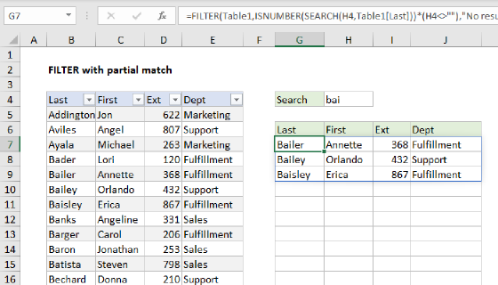
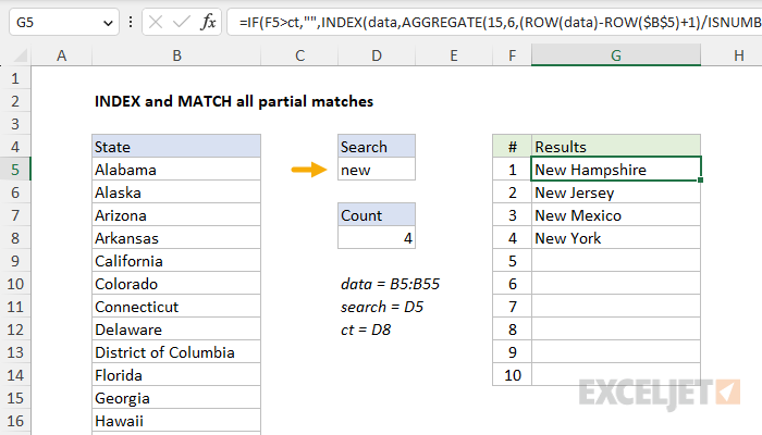
To extract all matches based on a partial match, you can use a formula based on the INDEX and AGGREGATE functions, with support from ISNUMBER and SEARCH. In the example shown, the formula in G5 is:
=IF(F5>ct,"",INDEX(data,AGGREGATE(15,6,(ROW(data)-ROW($B$5)+1)/ISNUMBER(SEARCH(search,data)),F5)))
where search (D5), CT (D8) and data (B5:B55) are named ranges.
Note: in the current version of Excel, the FILTER function is a better way to solve this problem. The INDEX and MATCH formula explained here is meant for legacy versions of Excel that do not provide the FILTER function.
Generic formula
=IF(F5>ct,"",INDEX(data,AGGREGATE(15,6,(ROW(data)-ROW($B$5)+1)/ISNUMBER(SEARCH(search,data)),F5)))
Explanation
Note: in the current version of Excel, the FILTER function is a better way to solve this problem. The INDEX and MATCH formula explained here is meant for legacy versions of Excel that do not provide the FILTER function.
The core of this formula is the INDEX function, with AGGREGATE used to figure out the "nth match" for each row in the extraction area:
INDEX(data,nth_match_formula)
Almost all of the work is in figuring out and reporting which rows in "data" match the search string, and reporting the position of each matching value to INDEX. This is done with the AGGREGATE function configured like this:
AGGREGATE(15,6,(ROW(data)-ROW($B$5)+1)/ISNUMBER(SEARCH(search,data)),F5)
The first argument, 15, tells AGGREGATE to behave like SMALL, and return nth smallest values. The second argument, 6, is an option to ignore errors. The third argument is an expression that generates an array of matching results (described below). The fourth argument, F5, acts like "k" in SMALL to specify the "nth" value.
AGGREGATE operates on arrays, and the expression below builds an array for the third argument inside AGGREGATE :
(ROW(data)-ROW($B$5)+1)/ISNUMBER(SEARCH(search,data))
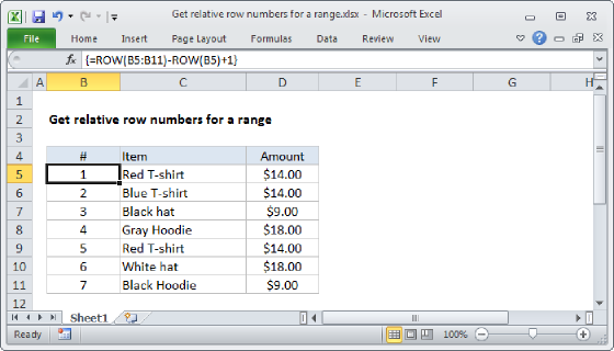
Here, the ROW function is used to generate an array of relative row numbers, and ISNUMBER and SEARCH are used together to match the search string against values in the data, which generates an array of TRUE and FALSE values.
The clever bit is to divide the row numbers by the search results. In a math operation like this, TRUE behaves like 1, and FALSE behaves like zero. The result is row numbers associated with a positive match are divided by 1 and survive the operation, while row numbers associated with non-matching values are destroyed and become #DIV/0 errors. Because AGGREGATE is set to ignore errors, it ignores the #DIV/0 errors, and returns the "nth" smallest number in the remaining values, using the number in column F for "nth".
Managing performance
Like all array formulas, this formula is "expensive" in terms of resources with a large data set. To minimize performance impacts, the entire INDEX and MATCH formula is wrapped in IF like this:
=IF(F5>ct,"",formula)
where the named range "ct" (D8) holds this formula:
=COUNTIF(data,"*"&search&"*")
This check stops the INDEX and AGGREGATE portion of the formula from executing once all matching values are extracted.
Array formula with SMALL
If your version of Excel does not have the AGGREGATE function, you can use an alternative formula based on SMALL and IF:
=IF(F5>ct,"",INDEX(data,SMALL(IF(ISNUMBER(SEARCH(search,data)),ROW(data)-ROW($B$5)+1),F5)))
Note: this is an array formula and must be entered with control + shift + enter.
FILTER function
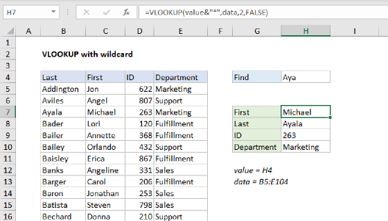
The INDEX and MATCH formula explained above is meant for legacy versions of Excel that do not offer the FILTER function. In the current version of Excel, a better way to solve this problem is to use FILTER in a formula like this:
=FILTER(data,ISNUMBER(SEARCH(search,data)))
As you can see, this is a much simpler formula. For a detailed explanation, see this page.