Summary
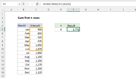
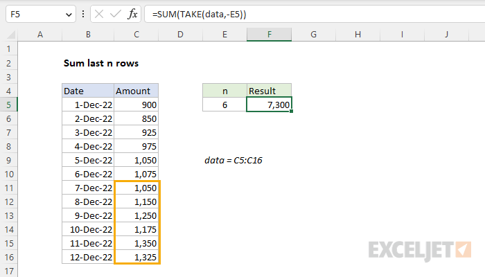
To sum the last n rows of values in a range, you can use the SUM function with the TAKE function. In the example shown, the formula in F5 is:
=SUM(TAKE(data,-E5))
Where data is the named range C5:C16. The result is 7,300, the sum of the last 6 values.
The TAKE function is new in Excel. See below for a formula that will work in older versions.
Generic formula
=SUM(TAKE(range,-n))
Explanation
In the example shown, we have a list of amounts in column C. The goal is to dynamically sum the last n amounts using the number that appears in cell E5 for n. Since the list may grow over time, the key requirement is to sum amounts by position. For convenience only, the values to sum are in the named range data (C5:C16). In the latest version of Excel, the best way to solve this problem is with the TAKE function, a new dynamic array function in Excel. In older versions of Excel, you can use the OFFSET function. Both approaches are explained below.
TAKE function
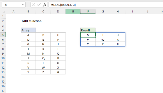
The TAKE function returns a subset of a given array. The number of rows and columns to return is provided by separate rows and columns arguments. For example, you can use TAKE to return the first 3 rows or columns of an array like this:
=TAKE(array,3) // first 3 rows
=TAKE(array,,3) // first 3 columns
A great feature of TAKE is that you can supply a negative value to retrieve last rows or columns:
=TAKE(array,-3) // last 3 rows
=TAKE(array,,-3) // last 3 columns
In this problem, we want to sum the last n values that appear in data, where the number of rows to return is a variable entered in cell E5. To retrieve these values, we can use TAKE like this:
TAKE(data,-E5)
With the number 6 in cell E5, TAKE will return an array with six values like this:
{1050;1150;1250;1175;1350;1325}
To sum these values, we simply need to nest the TAKE function inside the SUM function:
=SUM(TAKE(data,-E5))
=SUM({1050;1150;1250;1175;1350;1325})
=7300
The result is 7,300, the sum of the last six values in the range C5:C16. As new values are added to data, TAKE will continue to return the last n values to SUM.
Making the range dynamic
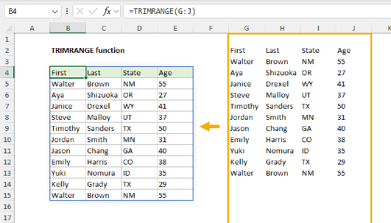
One limitation of the formula explained above is that it assumes that the range going into the TAKE function contains all data. What should you do if new data is being added on an ongoing basis? One easy solution is to use the TRIMRANGE function to create a simple dynamic range like this:
=SUM(TRIMRANGE(TAKE(range,-n)))
The TRIMRANGE function removes empty rows and columns from a range of data. The result is a "trimmed" range that only includes data from the used portion of the range. Because it is a formula, TRIMRANGE will update the range dynamically when data is added or removed from the original range. To make this work correctly, you will want to use a range that is largest enough to hold all possible data. For example, if the data is in column A, you can use a full-column reference like this:
=SUM(TRIMRANGE(TAKE(A:A,-n)))
With TRIMRANGE in the formula, TAKE will always get the latest data. You can read more about the TRIMRANGE function here.
OFFSET function
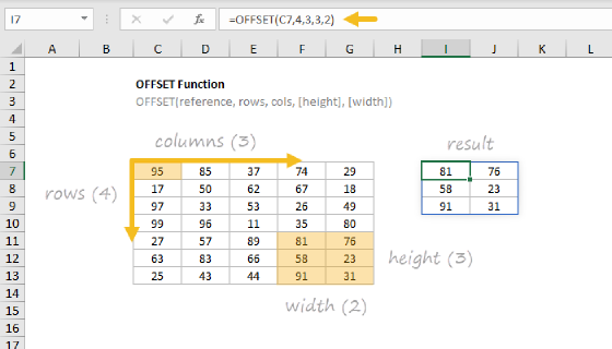
In older versions of Excel that do not have the TAKE function, you can use the OFFSET function to solve this problem. OFFSET is designed to create a reference for a range using five inputs: (1) a starting point, (2) a row offset, (3) a column offset, (4) a height in rows, (5) a width in columns. To sum the last 6 values in data (C5:C16), we can use the OFFSET function with the SUM function like this:
=SUM(OFFSET(C5,COUNT(data)-E5,0,E5))
Inside OFFSET, we use C5 for reference, since we want to start at C5. For rows, we use this snippet:
COUNT(data)-E5 // rows offset
Our goal is to create a range that starts at the cell in data that is n cells before last cell. The COUNT function returns the number of numeric values in data. We subtract E5 to "back up" to the correct cell. For cols, we provide 0 since we don't want a column offset. We provide E5 for height, since we want our final range to be n cells tall. We don't need to provide a value for the optional width argument, since width will inherit from reference. In this configuration, OFFSET will return a reference to C11:C16, which contains the last 6 values in data. The formula will evaluate like this:
=SUM(OFFSET(C5,COUNT(data)-E5,0,E5))
=SUM(OFFSET(C5,12-6,0,6))
=SUM(C11:C16)
=SUM({1050;1150;1250;1175;1350;1325})
=7300
The final result is 7300, the sum of the last six values in the range C5:C16.
INDEX function
One thing you might notice about the OFFSET formula above is that we are providing a reference to both data and cell C5, the first cell in data. This makes the formula more error-prone since data and C5 are disconnected. You can make the formula more robust and portable by using the INDEX function to return the first cell in data like this:
=SUM(OFFSET(INDEX(data,1),COUNT(data)-E5,0,E5))
This works because the INDEX function returns C5 as a reference, not a value. Now, as long as the reference to data is correct, the formula will work properly.
Making the range dynamic
One limitation of the formulas above is that they won't automatically include new data added to the range. In an older version of Excel, one way to make the range expand to include new data is to create a dynamic named range with a formula. You can create a dynamic named range with the OFFSET function or with the INDEX function. Another (simpler) option is to use an Excel Table to create the range.