Average last 3 numeric values

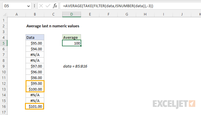
In this example, the goal is to average the last 3 numeric values in a set of data. The best solution depends on the version of Excel you have available. In the current version of Excel, this can be nicely solved with a formula based on the AVERAGE function, the FILTER function, and the TAKE function. In older versions of Excel, you can use an alternative formula based on the LOOKUP function, the LARGE function, and the ROW function. Both approaches are explained below.

Note: the difference in complexity between the modern formula and the legacy formula below is a great example of how new functions in Excel are making hard problems much easier to solve.

Modern formula

In the current version of Excel, which supports dynamic array formulas, you can solve this problem with a formula like this:

=AVERAGE(TAKE(FILTER(data,ISNUMBER(data)),-3))

Working from the inside out, the FILTER function is configured to extract only numeric values from the named range data (B5:B16) like this:

FILTER(data,ISNUMBER(data))

The ISNUMBER function creates the filtering logic. ISNUMBER returns TRUE for numeric values and FALSE for anything else. Because we are giving ISNUMBER a range that contains 12 values, ISNUMBER returns an array with 12 TRUE or FALSE values like this:

{TRUE;TRUE;FALSE;FALSE;TRUE;TRUE;TRUE;TRUE;TRUE;FALSE;FALSE;TRUE}

This array is returned to the FILTER function as the include argument, and FILTER returns only the 8 numeric values in data in an array like this:

{95;94;97;96;98;99;100;101}

This array above is handed off to the TAKE function, which is configured to return only the last 3 values:

TAKE({95;94;97;96;98;99;100;101},-3)

TAKE then returns 99, 100, and 101 to the AVERAGE function:

=AVERAGE({99;100;101})

AVERAGE calculates an average of the 3 values and returns 100 as a final result.

Variable n

The generic form of this formula where n is a variable is shown below. To change the number of numeric values being averaged, just change n to a different number.

=AVERAGE(TAKE(FILTER(data,ISNUMBER(data)),-n))

One nice thing about the TAKE function is that it will automatically handle the case where the number of requested values is greater than the number of values in the array returned by FILTER. For example, if you ask TAKE for 5 values, and there are only 3 values available, TAKE will return 3 values without an error.

Last n columns

Although the example shown has data in rows, the formula can be adjusted to work with data in columns like this:

=AVERAGE(TAKE(FILTER(data,ISNUMBER(data)),1,-n))

This formula assumes that values appear in columns. The only difference is that the 2nd argument in TAKE (rows) is now 1, and a 3rd argument (columns) has been added and set to -3. In other words, we are asking TAKE for the last n columns instead of the last n rows.

Legacy Excel

In Legacy Excel we need to take a different approach because we don't have the FILTER function or the TAKE function to use. One option is to use a formula like this:

=AVERAGE(LOOKUP(LARGE(IF(ISNUMBER(data),ROW(data)),{1,2,3}),ROW(data),data))

Notice the AVERAGE function is the outermost function in the formula. AVERAGE will calculate an average of numbers presented in an array, so almost all the work in this formula is to generate an array of the last 3 numeric values in a range. Working from the inside out, the IF function is used to "filter" numeric values:

IF(ISNUMBER(data),ROW(data))

The ISNUMBER function returns TRUE for numeric values, and FALSE for other values (including blanks), and the ROW function returns row numbers, so the result of this operation is an array of row numbers that correspond to numeric entries:

{5;6;FALSE;FALSE;9;10;11;12;13;FALSE;FALSE;16}

This array goes into the LARGE function with the array constant {1,2,3} for k:

LARGE({5;6;FALSE;FALSE;9;10;11;12;13;FALSE;FALSE;16},{1,2,3})

LARGE automatically ignores the FALSE values and returns an array with the largest 3 numbers, which correspond to the last 3 rows with numeric values:

{16,13,12}

This array goes into the LOOKUP function as the lookup value. The lookup array is provided by the ROW function, and the result array is the named range data (B5:B16):

LOOKUP({16,13,12},ROW(data),data)

After ROW runs, we have:

LOOKUP({16,13,12}, {5;6;7;8;9;10;11;12;13;14;15;16}, data)

LOOKUP locates the 3 row numbers in the array of row numbers returned by ROW, and returns the 3 corresponding values from data directly to the AVERAGE function:

=AVERAGE({101,100,99})

AVERAGE calculates an average of the 3 values and returns 100 as a final result.

Note: I ran into this clever approach over on chandoo.org, in a reply by Sajan to a similar question.

Making n variable

To make n variable so that it can be easily changed, you can replace the hardcoded array constant {1,2,3} with a dynamic array created with the INDIRECT function like this:

=AVERAGE(LOOKUP(LARGE(IF(ISNUMBER(data),ROW(data)),ROW(INDIRECT("1:"&n))), ROW(data), data))

Note that if the number of numeric values in data drops below n, this formula will return the #NUM error since LARGE won't be able to return 3 values as requested. To guard against this problem, you can use the MIN function like this:

ROW(INDIRECT("1:"&MIN(3,COUNT(data))))

Here, MIN is used to set the size of the requested array to n or the actual count of numeric values, whichever is smaller.