Average top 3 scores

Summary

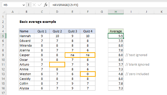
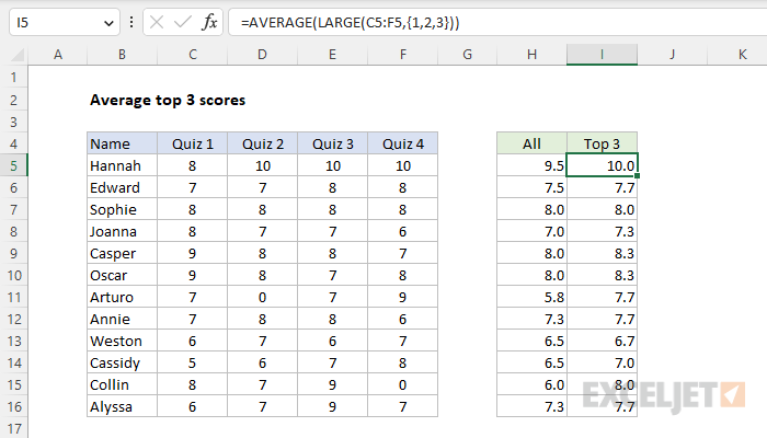
To average the top 3 scores in a set of data, you can use the AVERAGE function with the LARGE function. In the example shown, the formula in I5, copied down, is:

=AVERAGE(LARGE(C5:F5,{1,2,3}))

The result in cell I5 is 10, the average of the top 3 scores for Hannah. The average in H5 is 9.5 and includes all 4 quiz scores.

Generic formula

=AVERAGE(LARGE(range,{1,2,3}))

Explanation

In this example, the goal is to calculate an average of the top 3 quiz scores for each name listed in column B. For reference, column H has a formula that calculates an average of all 4 scores. This is a slightly tricky problem, because it's not obvious how to limit the scores included in the average to only the top 3 scores. The classic solution is to use the AVERAGE function with the LARGE function as explained below.

LARGE function

The LARGE function is designed to retrieve the "top nth value" from a set of numbers. For a given range, LARGE(range,1) will return the largest value, LARGE(range,2) will return the 2nd largest value, and so on, as seen below:

LARGE(range,1) // 1st largest value
LARGE(range,2) // 2nd largest value
LARGE(range,3) // 2nd largest value

In this problem, we need to configure LARGE to retrieve the largest 3 values, and the easiest way to do that is to pass an array constant like {1,2,3} into LARGE as the second argument, k. Because we are asking for the top 3 values, LARGE will return an array that contains all 3 values:

LARGE(range,{1,2,3}) // largest 3 values

LARGE with AVERAGE

In the example shown, the formula in cell I5 is:

=AVERAGE(LARGE(C5:F5,{1,2,3}))

Working from the inside out, the LARGE function is configured to extract the top 3 scores from the range C5:F5 like this:

LARGE(C5:F5,{1,2,3}) // returns {10,10,10}

Because we have provided the array constant {1,2,3} for the second argument, k, LARGE returns the top 3 scores in C5:F5 in an array like this:

{10,10,10}

This array is returned directly to the AVERAGE function:

=AVERAGE({10,10,10}) // returns 10

The AVERAGE function then returns the average of these values as a final result. As the formula is copied down, it returns an average of the top 3 scores for each name in the list. Although this set of data contains only 4 scores, the formula will work correctly for any number of scores, as long as there are at least 3.

Variable n

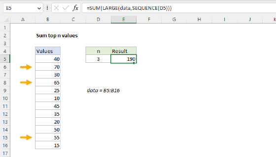
To make this formula use a variable for n, where n represents the number of values to include in the average, you can add the SEQUENCE function like this:

=AVERAGE(LARGE(C5:F5,SEQUENCE(n)))

To supply a value for n, you can use a cell reference like A1 or simply hardcode a number into the formula. The SEQUENCE function dynamically generates a numeric array which is then returned to LARGE as the second argument, and the formula works the same thereafter.

Legacy Excel

In Legacy Excel, the SEQUENCE function does not exist. The classic solution for creating a numeric array in older versions of Excel is to use the ROW and INDIRECT functions. For example, to generate a numeric array from 1 to 10, you can use a formula like this:

=ROW(INDIRECT("1:10")) // returns {1;2;3;4;5;6;7;8;9;10}

The INDIRECT function converts the text string "1:10" to the range 1:10, which is returned to the ROW function. ROW then returns an array of row numbers like {1;2;3;4;5;6;7;8;9;10}. To make n variable, you can concatenate the string "1:" to a cell reference that provides a value for n:

=AVERAGE(LARGE(C5:F5,ROW(INDIRECT("1:"&n))))

Note that this formula is an array formula and must be entered with control + shift + enter in older versions of Excel.