Summary
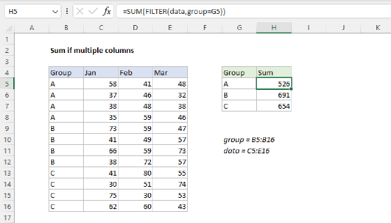
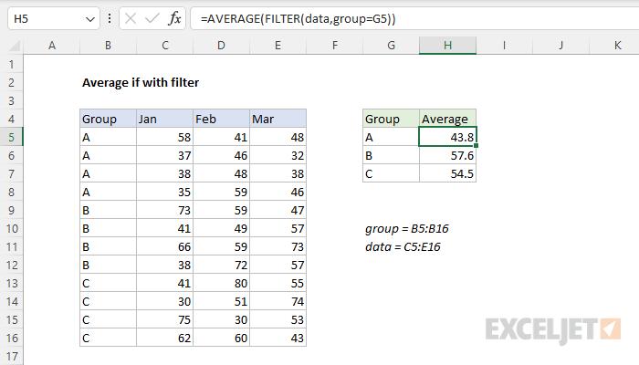
To calculate a conditional average for multiple columns of data, you can use the AVERAGE function with the FILTER function. In the worksheet shown, the formula in cell H5 is:
=AVERAGE(FILTER(data,group=G5))
where data (C5:E16) and group (B5:B16) are named ranges. The result is the average of values in group "A" for all three months of data. As the formula is copied down, it calculates an average for each group in column G. The FILTER function is a new function in Excel. See below for alternatives that will work in older versions of Excel.
Note: I was inspired to create this example after watching a good video by Excel expert Chandoo.
Generic formula
=AVERAGE(FILTER(data,group=A1))
Explanation
In this example, the goal is to calculate an average for any given group ("A", "B", or "C") across all three months of data in the range C5:E16. For convenience only, data (C5:E16) and group (B5:B16) are named ranges. In the article below, we look at several approaches to this problem:
- Why the AVERAGEIFS function won't work.
- A solution based on AVERAGE + FILTER
- A solution based on AVERAGE + IF function
- A solution based on SUMPRODUCT and Boolean algebra
In the latest version of Excel, the FILTER option (#2) is easy and intuitive. In Legacy Excel, you can use solution #3 or #4.
AVERAGEIFS won't work
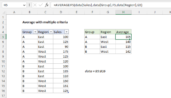
You might be tempted to solve this problem with the AVERAGEIFS function. After all, it seems to fit the bill. We simply need to calculate an average for a range of data based on one condition: we need to check if group (B5:B16) is equal to "A" or "B" or "C". In fact, we can easily use AVERAGEIFS to calculate an average for a given group on one month of data. For example, to calculate an average for group "A" in January, we can use a formula like this:
=AVERAGEIFS(C5:C16,group,"A") // returns 42
However, if we try to expand average_range to include all three columns in data (C5:E16), we'll get a #VALUE! error:
=AVERAGEIFS(data,group,"A") // returns #VALUE!
Why? The reason is that AVERAGEIFS expects average_range to be the same size as criteria_range. When we try to use the 1-column range group (B5:B16) with the 3-column range data (C5:E16), AVERAGEIFS returns an error. Incidentally, if we give the older AVERAGEIF function the entire data range and the same criteria, we don't get an error, but we do get an incorrect result:
=AVERAGEIF(group,"A",data) // returns 42
This happens because AVERAGEIF makes certain assumptions about average_range, essentially resizing it to match the range argument, using the upper left cell in the range as an origin. It's worth noting that this kind of "silent failure" is dangerous, in that the result seems reasonable but is in fact incorrect. You may not like formula errors, but at least they tell you something is wrong.
AVERAGE with FILTER
In the latest version of Excel, a good solution in this case is to use the AVERAGE function with the FILTER function. This is the approach used in the worksheet shown, where the formula in cell H5, copied down, is:
=AVERAGE(FILTER(data,group=G5))
And data (C5:E16) and group (B5:B16) are named ranges. Inside the AVERAGE function, the FILTER function is configured to filter the data in C5:E16 with a simple logical expression:
FILTER(data,group=G5)
Because cell G5 contains "A", and group (B5:B16) contains 12 values, the expression returns an array with 12 TRUE and FALSE values like this:
{TRUE;TRUE;TRUE;TRUE;FALSE;FALSE;FALSE;FALSE;FALSE;FALSE;FALSE;FALSE}
Notice the first four values in the array are TRUE, which corresponds to the first 4 rows in the data, which are in group A. This array is returned to the FILTER function as the include argument, and FILTER uses this array to select the first 4 rows of data (C5:E16).
The result from FILTER is delivered directly to the AVERAGE function as a single array:
=AVERAGE({58,41,48;37,46,32;38,48,38;35,59,46})
AVERAGE returns a final result of 43.8, the average of the 12 numbers in the array returned by FILTER. As the formula is copied down, it calculates an average for each group, using the value in column G for group.
AVERAGE with IF
The FILTER function is a newer function that does not exist in Legacy Excel. If you are using an older version of Excel, you can solve this problem with a simple array formula like this:
{=AVERAGE(IF(group=G5,data))}
In this formula, we use the IF function to filter values in each group instead of FILTER. When the value in group matches the value in G5 ("A"), IF returns the corresponding values in data. When a value doesn't match, IF returns FALSE for corresponding values in data. After IF is evaluated, the array of results returned to AVERAGE looks like this:
=AVERAGE({58,41,48;37,46,32;38,48,38;35,59,46;FALSE,FALSE,FALSE;FALSE,FALSE,FALSE;FALSE,FALSE,FALSE;FALSE,FALSE,FALSE;FALSE,FALSE,FALSE;FALSE,FALSE,FALSE;FALSE,FALSE,FALSE;FALSE,FALSE,FALSE})
This works because the AVERAGE function will automatically ignore the logical values TRUE and FALSE. This is an array formula and must be entered with control + shift + enter in older versions of Excel.
One thing to be aware of with this approach is that empty cells will be treated as zero, and become part of the calculated average. This happens because when the empty cells get passed through the IF function, they become zero (0). Although the AVERAGE function will ignore empty values, it will include zero (0) values in the calculated average. To avoid this problem, you can add a second IF function to test for empty values like this:
{=AVERAGE(IF(group=G5,IF(data<>"",data)))}
In this formula, only values that are part of group "A" and are not empty are passed into the AVERAGE function. All other values become FALSE and are ignored by the AVERAGE function.
Both formulas above are array formulas and must be entered with control + shift + enter in older versions of Excel. In the current version of Excel, which supports array formulas natively, the formulas will "just work".
SUMPRODUCT function
As you might guess, you can also use the flexible SUMPRODUCT function to solve this problem in older versions of Excel. The formula looks like this:
=SUMPRODUCT(--(group=G5)*data)/SUMPRODUCT(--(group=G5)*(data<>""))
In this formula, the first SUMPRODUCT calculates a sum of all data in group "A" (from cell G5):
=SUMPRODUCT(--(group=G5)*data) // sum (526)
The second SUMPRODUCT calculates a count of all data in the same group:
SUMPRODUCT(--(group=G5)*(data<>"")) // count (12)
After both SUMPRODUCT formulas are evaluated, the final step is to divide the sum by the count:
=SUMPRODUCT(--(group=G5)*data)/SUMPRODUCT(--(group=G5)*(data<>""))
=526/12
=43.8
Although slightly more complicated, the SUMPRODUCT formula does not need to be entered in a special way with control + shift + enter, since SUMPRODUCT can handle array operations natively.