=GROUPBY(row_fields, values, function, [field_headers], [total_depth], [sort_order], [filter_array], [field_relationship])- row_fields - The values for grouping.
- values - The values to aggregate.
- function - The calculation to run when aggregating.
- field_headers - [optional] 0 = No, 1 = Yes, don't show, 2 = No, generate, 3 = Yes, show.
- total_depth - [optional] Totals and subtotals. 0 = No, 1 = Grand Totals, 2 = Both, -1 = Grand Totals at top, -2 = Both at top.
- sort_order - [optional] Sort by index number. Negative numbers = descending order.
- filter_array - [optional] Logic to exclude specific rows.
- field_relationship - [optional] Field relationship when multiple columns are provided as row fields. 0 = Hierarchy (default), 1 = Table.
Using the GROUPBY function
The GROUPBY function is designed to summarize data by grouping rows and aggregating values. The result is a dynamic summary table created with a single formula. The output from the GROUPBY function is similar to the output from a Pivot Table, but without formatting. The summary returned by the GROUPBY function is fully dynamic and will immediately recalculate when source data changes. Here is a brief list of GROUPBY features and limitations:
- A simple and flexible way to make a summary table with a formula.
- Can apply aggregation functions like SUM, AVERAGE, COUNT, COUNTA, etc.
- Does not require a Pivot Table or helper columns.
- Can group by more than one level (i.e., Region and Color, etc.).
- Returns a dynamic array that automatically updates when data changes.
- Able to exclude specific rows in the source data with logical expressions.
- Does not apply formatting; you must apply formatting manually.
- Only available in Excel 365.
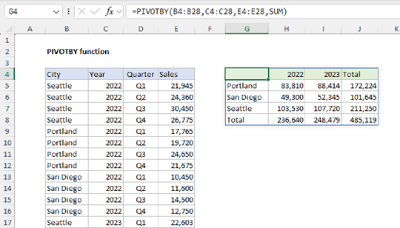
The GROUPBY function is similar to the PIVOTBY function. The difference is that PIVOTBY can group by row and column, whereas GROUPBY can group by row only.
Table of Contents
- GROUPBY basic example
- GROUPBY with field headers
- GROUPBY calculation options
- GROUPBY with multiple calculations
- GROUPBY with custom headers
- GROUPBY with multiple columns
- GROUPBY total options
- GROUPBY sort options
- GROUPBY with filter array
- GROUPBY with field relationships
- GROUPBY with custom LAMBDA
- GROUPBY with a dynamic range
GROUPBY basic example
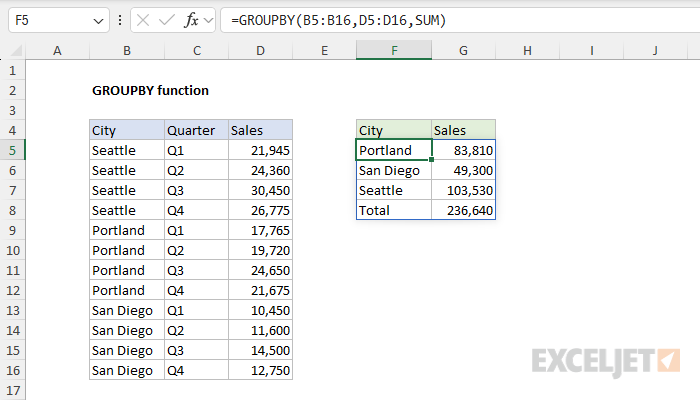
The GROUPBY function takes eight arguments, but only the first three are required. In the worksheet below, we use the GROUPBY function to summarize Sales by City. The formula in cell F5 is:
=GROUPBY(B5:B16,D5:D16,SUM)
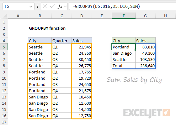
For this example, GROUPBY is configured with three arguments as follows:
- row_fields - provided as the range B5:B16, which contains city names.
- values - provided as the range D5:D16, which contains sales amounts.
- function - provided as SUM, the calculation to perform during aggregation.
With the inputs above, the GROUPBY function sums Sales by City and outputs the table in F4:G8 in one step. Notice that we have not included the header row in row_fields or values, because we are not asking GROUPBY to generate a header automatically. Instead, we have manually entered a header row in F4:G4. Also note that GROUPBY includes a Total row by default. In the example below, we'll look at how to configure GROUPBY to output field headers in the source data.
GROUPBY with field headers
The fourth argument in GROUPBY, field_headers, controls how the header row is handled when it is part of the data provided to the GROUPBY function. There are five possible values for field_headers:
| Value | Meaning |
|---|---|
| Automatic header detection (default). | |
| 0 | Headers are not provided in the data. |
| 1 | Headers are included, but should not be displayed. |
| 2 | Headers are not included but should be generated. |
| 3 | Headers are included and should be displayed. |
The field_headers argument is optional. When field_headers is omitted, GROUPBY will automatically detect headers in the source data by testing values. If the first value is text and the second value is numeric, GROUPBY will assume the first row contains headers. You can see the automatic detection behavior in the example above, where the ranges used for row_fields and values do not include the header row. Because the first value is numeric (not text), GROUPBY assumes that headers are not part of the source data (which is correct). However, automatic detection only prevents the headers from being processed as values; it does not display headers. To display field headers in source data, you must specifically enable them by setting field_headers to 3. You can see how this works in the example below, where the ranges provided for row_fields and values include a header row, and field_headers is provided as 3:
=GROUPBY(B4:B16,D4:D16,SUM,3) // field headers enabled
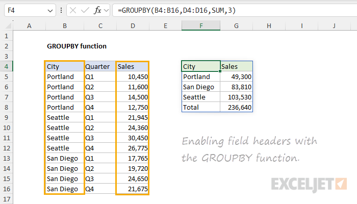
The inputs to GROUPBY are as follows:
- row_fields - provided as the range B4:B16, which contains city names, plus the header row.
- values - provided as the range D4:D16, which contains sales amounts, plus the header row.
- function - provided as SUM, the calculation to perform during aggregation.
- field_headers - provided as 3, since the data now includes a header row that should be displayed.
Note that the data in this example is the same as the previous example. However, the ranges used for row fields and values now include the headers in row 4. As a result, the formula is entered in cell F4 instead of F5 to keep the output table in the same location.
GROUPBY calculation options
The third argument in GROUPBY is function, which specifies the calculation to perform when values are grouped. Available calculations include Excel functions like SUM, COUNT, COUNTA, MAX, MIN, etc. The function is called with eta lambda syntax, which is just the function name, without parentheses and arguments. In the worksheet below, we have a list of meal preferences for 100 employees in different departments and the cost per meal. We can use the GROUPBY function to analyze this data in a variety of ways. In the first example below, we use GROUPBY to generate a count for each meal (Beef, Chicken, and Veggie). In this case, we want to count the meals, which are text values, so we provide COUNTA for function. The formula in G5 looks like this:
=GROUPBY(D4:D104,D4:D104,COUNTA,1)
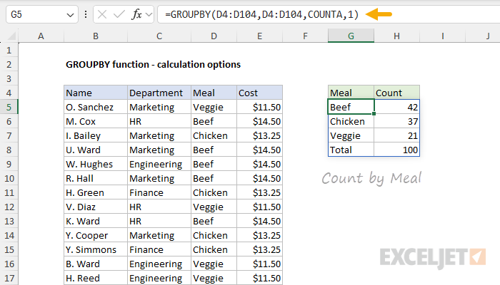
- row_fields - D4:D104 (Meal), because we want to group by meal.
- values - D4:D104 (Meal) because we want to count meals.
- function - COUNTA, because we want to count text values.
- field_headers - 1, because the data contains a header row we don't want to display.
Note: Field headers are included in the source data ranges, but we don't want to display field headers because we want to use the word "Count" for the counted meals in cell H4. As a result, we provide 1 for field_headers.
In the next example, we've changed the calculation to generate a total cost by meal, as seen below. The formula in G5 now looks like this:
=GROUPBY(D4:D104,E4:E104,SUM,1)
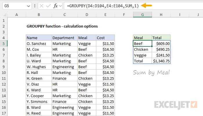
- row_fields - D4:D104 (Meal), because we want to group by meal.
- values - E4:E104 (Cost) because we want to sum cost.
- function - SUM, because we want to provide a total.
- field_headers - 1, because the data contains a header row we don't want to display.
Note: Here again, we don't want to display field headers because we want to use the word "Total" in H4, so we provide 1 for field_headers.
GROUPBY with multiple calculations
It is possible to perform more than one calculation with GROUPBY, but it is not obvious how to do so, since the function argument accepts just one value. The trick is to use the HSTACK function inside GROUPBY to call more than one function simultaneously. For example, in the worksheet below, we are using GROUPBY to count by meal and sum by meal at the same time. The formula in G4 looks like this:
=GROUPBY(D4:D104,E4:E104,HSTACK(COUNT,SUM),1)
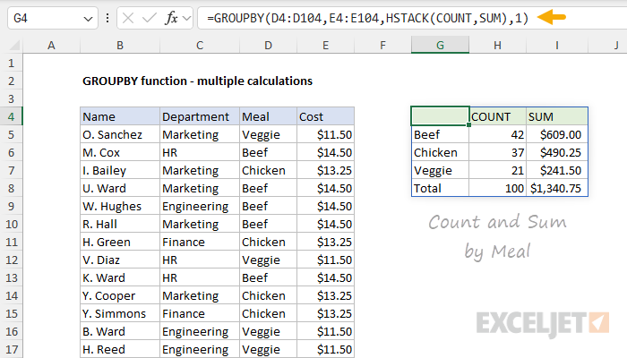
- row_fields - D4:D104 (Meal), because we want to group by meal.
- values - E4:E104 (Cost), because we want to sum the cost.
- function - HSTACK(COUNT,SUM), because we want to count and sum.
- field_headers - 1, because the data contains a header row we don't want to display.
Notice that the formula is now entered in cell G4, even though we have set field_headers to 1 (do not display). This is because GROUPBY automatically adds column headers when you ask for multiple calculations. As a result, we have COUNT in H4 and SUM in I4. Cell G4 is blank because we have disabled field headers. To perform another calculation, just add the function name to the values inside HSTACK. In the example below, we have added the PERCENTOF function to HSTACK, and the formula in G4 is now:
=GROUPBY(D4:D104,E4:E104,HSTACK(COUNT,SUM,PERCENTOF),1)
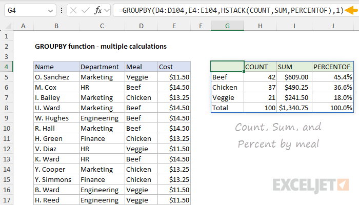
Note that the formatting in the table seen above has been applied manually. Also, note that the structure of the table is not ideal. The first column lacks a header, and the function names used for calculations are a bit clunky. See below for a workaround.
When adding the PERCENTOF function as a function inside GROUPBY, you must take care that you are providing numeric values. If the values are text, PERCENTOF will return #DIV/0!. For a detailed explanation, see: GROUPBY with survey results.
GROUPBY with custom headers
When you add multiple calculations to the GROUPBY function, you automatically get headers on the calculated columns. Depending on your use case, you may want to override these headers and supply your own custom values. To do that, you can remove the headers with the DROP function and add your own with the VSTACK function. You can see an example of this in the example below, which performs three calculations: COUNT, SUM, PERCENTOF. The formula in cell G4 looks like this:
=VSTACK(
{"Meal","Count","Cost","%"},
DROP(GROUPBY(D4:D104,E4:E104,HSTACK(COUNT,SUM,PERCENTOF),1),1)
)
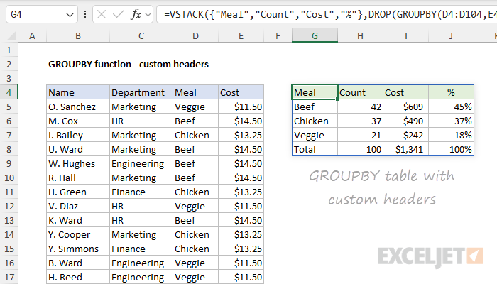
- Inside the DROP function, we have the original GROUPBY formula.
- DROP removes the header row and passes the result into VSTACK.
- VSTACK stacks the custom headers on top of the remaining table.
Note that the headers in G4:J4 come from custom values supplied as an array constant like {"Meal","Count","Cost","%"}. You are free to customize these values as you like.
In this example, we did extra work in order to get an all-in-one formula that returned both headers and data at the same time. However, a hybrid approach would be to enter the header row manually and then use DROP + GROUPBY alone to return just the table data without headers.
GROUPBY with multiple columns
The GROUPBY function can handle multiple columns for row_fields and values arguments. When you include multiple columns, the output will have multiple row group levels. To illustrate how this works, consider the examples below. In the first example, we provide one column for row_fields, and 1 column for values. The formula in G4 looks like this:
=GROUPBY(C4:C226,E4:E226,SUM,3)
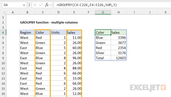
The inputs to GROUPBY are as follows:
- row_fields - Color (C4:C226), including the header row.
- values - Sales (E4:E226), including the header row.
- function - SUM to generate a total for each color.
- field_headers - 3, since the source data includes a header row that should be displayed.
With this configuration, GROUPBY groups Sales by Color and generates a total for Red, Green, Blue, and Silver as shown above. In the example below, we've modified the formula to include Region and Color for row_fields:
=GROUPBY(B4:C226,E4:E226,SUM,3)
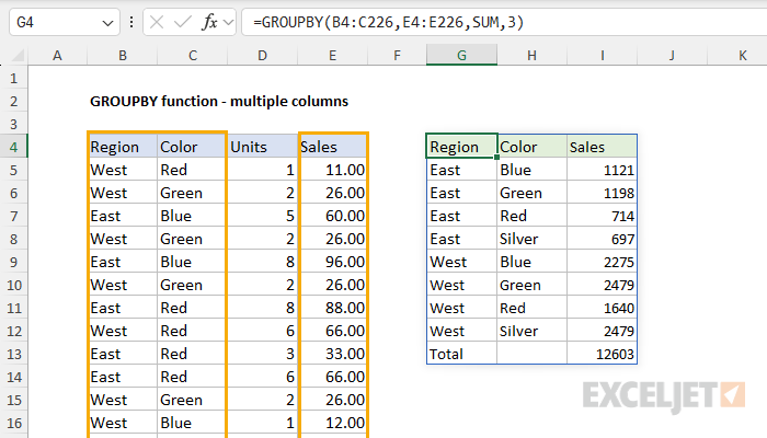
- row_fields - Region and Color (B4:C226), including the header row.
- values - Sales (E4:E226), including the header row.
- function - SUM to generate a total for each region/color.
- field_headers - 3, since the source data includes a header row that should be displayed.
The result is that GROUPBY groups Sales by Region and Color, and returns total Sales for each combination. Values can also be supplied as a range with more than one column. In the example below, row fields and values are provided as ranges that include two columns. The formula in G4 is:
=GROUPBY(B4:C226,D4:E226,SUM,3)
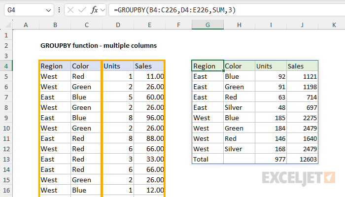
- row_fields - Region and Color (B4:C226), including the header row.
- values - Units and Sales (D4:E226), including the header row.
- function - SUM to generate totals for each region/color.
- field_headers - 3, since the source data includes a header row that should be displayed.
Here, we modified the Values range to include both Units and Sales. In this configuration, the GROUPBY function generates two totals for each Region/Color combination: a total for Units and a total for Sales.
GROUPBY total options
The fifth argument in GROUPBY, total_depth, controls how the totals are displayed in the output. Total_depth is an optional argument. When not provided, GROUPBY will automatically display grand totals. The table below shows possible settings for total_depth:
| Value | Meaning |
|---|---|
| Automatic grand totals (default). | |
| 0 | Do not display totals. |
| 1 | Display Grand Totals. |
| 2 | Display Grand Totals and Subtotals. |
| -1 | Display Grand Totals at top. |
| -2 | Display Grand Totals and Subtotals at top. |
By default, GROUPBY will create and display grand totals when total_depth argument is not provided. You can see how this works below, where the formula in cell G4 looks like this:
=GROUPBY(B4:C226,E4:E226,SUM,3) // total depth not provided
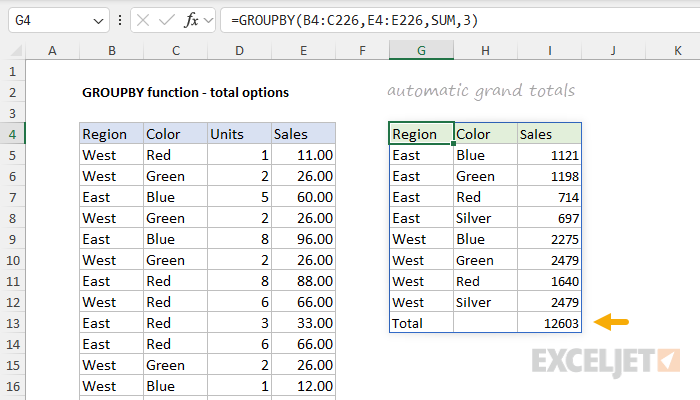
- row_fields - Region and Color (B4:C226), including the header row.
- values - Sales (E4:E226), including the header row.
- function - SUM to generate totals for Sales
- field_headers - 3, since the source data includes a header row that should be displayed.
- total_depth - not provided.
Note that the total in cell I13 is displayed by default. If we explicitly enable grand totals by setting total_depth to 1, we get the same result:
=GROUPBY(B4:C226,E4:E226,SUM,3,1) // total depth = 1
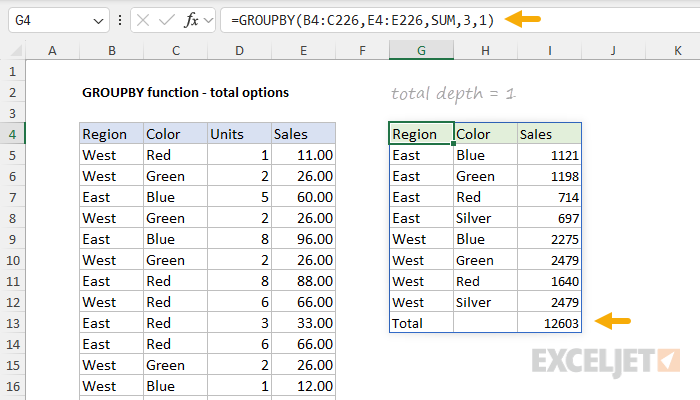
- row_fields - Region and Color (B4:C226), including the header row.
- values - Sales (E4:E226), including the header row.
- function - SUM to generate totals for Sales
- field_headers - 3, since the source data includes a header row that should be displayed.
- total_depth - 1, to explicitly enable a grand total.
Setting total_depth to 2 enables both grand totals and subtotals, as shown in the example below:
=GROUPBY(B4:C226,E4:E226,SUM,3,2) // total depth = 2
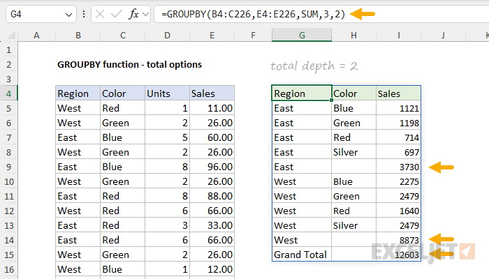
- row_fields - Region and Color (B4:C226), including the header row.
- values - Sales (E4:E226), including the header row.
- function - SUM to generate totals for Sales
- field_headers - 3, since the source data includes a header row that should be displayed.
- total_depth - 2, to enable subtotals and grand totals.
Now we have subtotals for Region in cells I9 and I14, and a grand total in cell I15.
For subtotals to display, row_fields must have at least 2 columns. If you try to enable subtotals when row_fields contains just one column, GROUPBY will return a #VALUE! error. It is possible to provide numbers greater than 2 for total_depth as long as row_fields has enough columns to support the requested total depth.
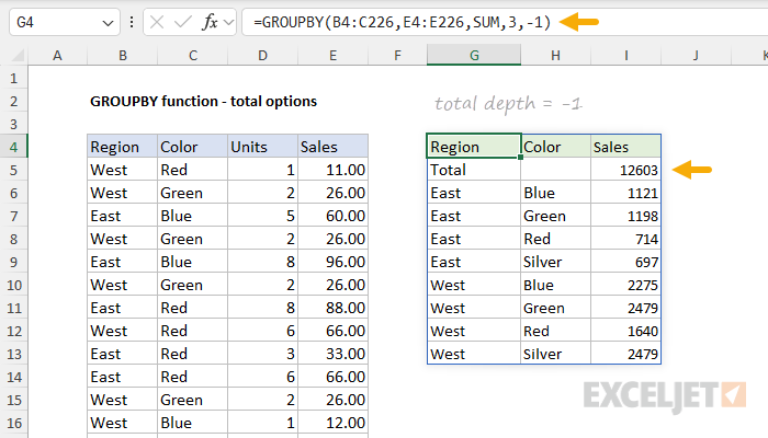
The GROUPBY function also supports displaying grand totals and subtotals at the top of a group instead of at the bottom. The example below moves grand totals to the top by setting total_depth to -1:
=GROUPBY(B4:C226,E4:E226,SUM,3,-1) // total depth = -1
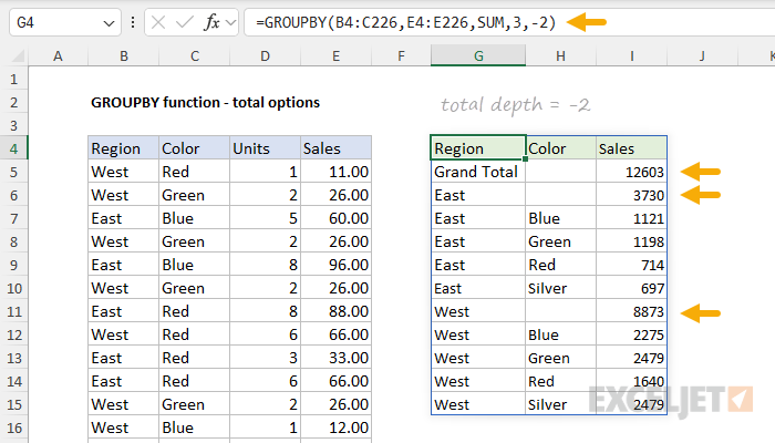
Likewise, subtotals can also be displayed at the top of a group by setting total_depth to -2:
=GROUPBY(B4:C226,E4:E226,SUM,3,-2) // total depth = -2
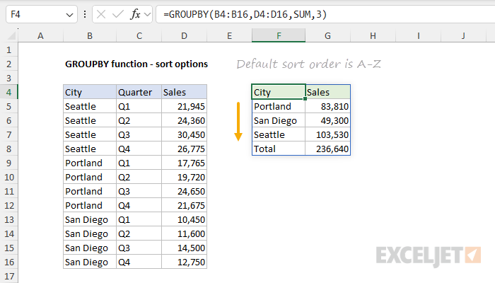
GROUPBY Sort options
By default, the GROUPBY function will sort values in standard ascending (A-Z) order, beginning with the leftmost row field. You can see this behavior in the example below, where no sort order has been specified and the table returned by GROUPBY is sorted A-Z by city name. The formula in cell F4 looks like this:
=GROUPBY(B4:B16,D4:D16,SUM,3) // no sort order specified
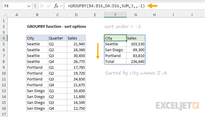
To override the default sort order, provide a value for the sort_order argument, which is given as an index number that can be positive (A-Z) or negative (Z-A). The number itself corresponds to the columns in the table, starting with 1 for the first column. For example, to sort the table by city name in descending (Z-A) order, use -1:
=GROUPBY(B4:B16,D4:D16,SUM,3,,-1) // sort city names Z-A
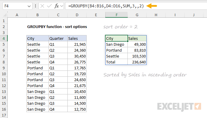
To sort the table by Sales in ascending order, provide a 2 for sort_order, where 2 means the second column:
=GROUPBY(B4:B16,D4:D16,SUM,3,,2)
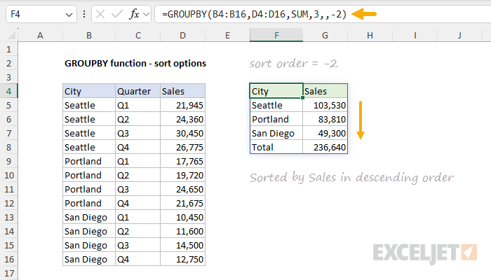
To sort the table by Sales in descending order, provide a -2 for sort_order, where the 2 means the second column and the negative sign (-) specifies a descending (Z-A) sort:
=GROUPBY(B4:B16,D4:D16,SUM,3,,-2)
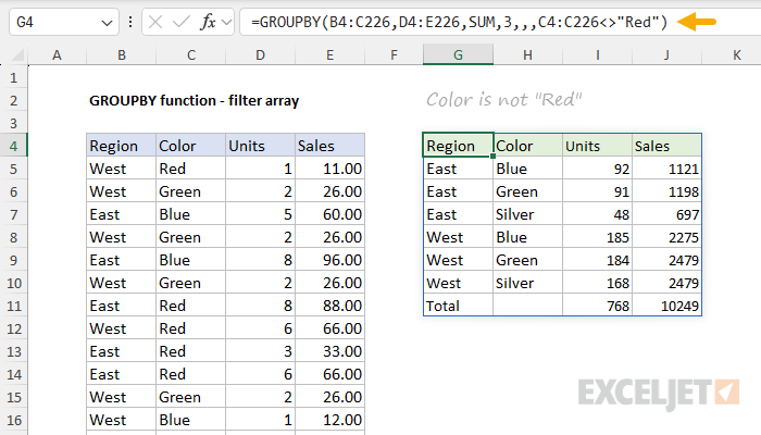
GROUPBY with filter array
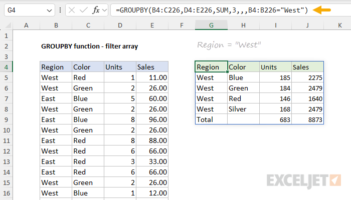
One of the interesting options available for the GROUPBY function is the ability to filter incoming data to include or exclude specific values. The optional filter_array argument controls this feature. When provided, filter_array is expected to be a single column of Booleans (i.e., TRUE and FALSE, or 1s and 0s) that indicate whether the corresponding row in the data should be included. These Booleans are typically generated with a logical expression. For example, in the workbook below, the data has been filtered to allow only rows corresponding to the West Region by providing the logical expression B4:B226="West" for filter_array. The formula in G4 looks like this:
=GROUPBY(B4:C226,D4:E226,SUM,3,,,B4:B226="West")
Note that filter_array should be the same length as the incoming data. In the example above, we match B4:B226 to the ranges used for row and value fields. The logic can be easily modified. To exclude all rows where the color is "Red", we can use a formula like this:
=GROUPBY(B4:C226,D4:E226,SUM,3,,,C4:C226<>"Red")
The logic for filter_array can be any expression that generates a correctly sized array of Booleans, and there are many ways to do this with Excel formulas and functions. We could, for example, use the REGEXTEST function to include rows where the color is "Red" or "Blue" in a formula like this:
=GROUPBY(B4:C226,D4:E226,SUM,3,,,REGEXTEST(C4:C226,"Red|Blue"))
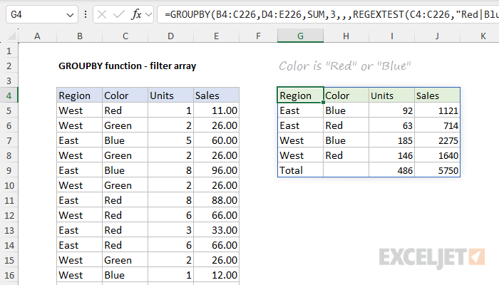
Regex is a newer feature in Excel. For a general introduction, see Regular Expressions in Excel.
GROUPBY and field relationships
The field_relationship argument specifies the "relationship" between fields when multiple columns are provided as row fields. There are two possible values: 0 = Hierarchy and 1 = Table. The default value is 0 (Hierarchy). Field relationship affects the way sorting works, but only when row_fields includes multiple columns. By default, GROUPBY uses a hierarchical relationship between row fields, which means that row fields sort from left to right. In other words, the sorting of additional row fields is controlled by the hierarchy of previous columns. When field_relationship is set to 1, the sorting of each field column works independently.
In the example below, we use the field_relationship argument (set to 1) to disable the hierarchy and allow the months to sort correctly using the month numbers created by the MONTH function. The formula in G5 looks like this:
=CHOOSECOLS(GROUPBY(HSTACK(TEXT(data[Date],"mmm"),MONTH(data[Date])),data[Total],SUM,,,2,,1),{1,3})
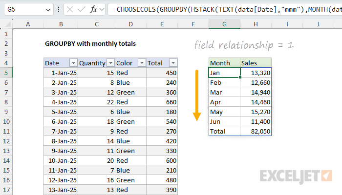
For a full tear-down of this formula and a detailed explanation of why the field relationship setting is required, see this page.
Note that when the field relationship is set to Table, subtotals are not supported because they rely on a hierarchy to work correctly.
GROUPBY with custom LAMBDA
The calculation performed by the GROUPBY function can be called in two different ways: (1) a short-form "eta lambda syntax" or (2) a long-form syntax that uses a custom LAMBDA function. For example, to group and sum values, the short-form syntax looks like this:
=GROUPBY(row_fields,values,SUM)
The long-form custom syntax for the same calculation looks like this:
=GROUPBY(row_fields,LAMBDA(x,SUM(x)))
Both formulas above will return the same result. Why two syntax options? The short form is for convenience. It is concise and easy to read. However, the behavior cannot be customized. The long-form syntax uses the LAMBDA function and can be customized as needed to apply a more advanced calculation. To illustrate this concept, suppose you want the round values that GROUPBY returns to the nearest 1000. We can use the ROUND function to round to the nearest 1000 like this:
=ROUND(number,-3)
But how do we get this into the GROUPBY function, which needs to sum the values before rounding them? The trick is to switch to the long-form LAMBDA syntax and use a calculation like this:
LAMBDA(x,ROUND(SUM(x),-3))
The core of this calculation is the long-form syntax LAMBDA(x,SUM(x), plus the ROUND function. The grouped values are passed into SUM, which returns the sum of a given group directly to ROUND, which rounds the number to the nearest 1000. The GROUPBY function then returns the rounded sum in the final output. You can see an example of this formula in action in the worksheet below, where the formula in cell F4 looks like this:
=GROUPBY(B4:B16,D4:D16,LAMBDA(x,ROUND(SUM(x),-3)),3)
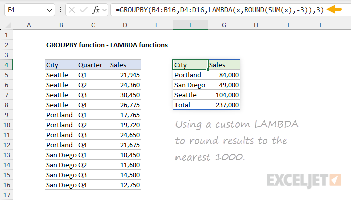
The ROUND example above is just for illustration. Because GROUPBY supports a custom LAMBDA function, you can perform any calculation that makes sense in the context of the GROUPBY function. See another example here.
GROUPBY with a dynamic range
When you use the GROUPBY function with data that changes frequently, you will probably want to configure it to use a dynamic range. A dynamic range is a range that expands and contracts as rows are added or removed. You have two good options to make the range: converting the data to an Excel Table, or using the TRIMRANGE function to create a dynamic named range. In both cases, you will then need to feed specific columns of the range into GROUPBY. With Excel Tables, this is easy, since you can refer to table columns by name. With a named range, you can use the CHOOSECOLS function to access specific columns and, if desired, you could give those columns names by wrapping the formula in the LET function, then feeding the column names into GROUPBY.