Summary
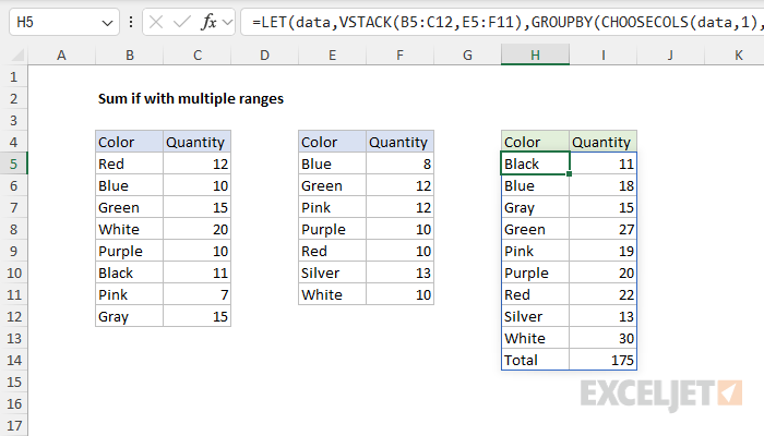
To sum multiple ranges with conditional logic (sum if), you can use the VSTACK function to combine the ranges and then use various other functions with the combined range to calculate conditional sums. In the worksheet shown, the goal is to calculate a total quantity for each color across the two ranges. This is done with the VSTACK function and the GROUPBY function. The formula in H5 looks like this:
 =LET(
data,VSTACK(B5:C12,E5:F11),
GROUPBY(CHOOSECOLS(data,1),CHOOSECOLS(data,2),SUM)
)
VSTACK combines the two ranges, and the GROUPBY function is used to sum quantities by color.
The formula above requires Excel 365 since VSTACK, LET, GROUPBY, and CHOOSECOLS are new functions. The article below explains how to accomplish the same thing using the SUMIFS function and a more manual approach.
Explanation
In this example, the goal is to calculate a total quantity for each color across the two ranges shown in the worksheet. The two ranges are "non-contiguous", which means they are not connected or touching. Both ranges contain a list of colors in the first column and quantities in the second column. Although we have just two ranges in this example, we want an approach that will scale to handle more ranges. Traditionally, this is a tricky problem in Excel because functions like SUMIFS aren't made to accept more than one range. Let's walk through some options step by step.
Using the SUM function
The SUM function can handle non-contiguous ranges natively. For example, if we simply want to return the total quantity of items in both ranges, we can use SUM in a formula like this:
=SUM(C5:C12,F5:F11) // returns 175
The result is 175, the total number of items in both ranges. However, things get more complicated if we want to perform a conditional sum. For example, what if we want to sum the quantity of "red" or "green" items in both ranges? This would normally be a job for the SUMIF or SUMIFS function.
Using the SUMIFS function
The traditional approach to a problem like this is to use the SUMIFS function more than once and then add the results together. For example, here is how we would set things up to get a total for "red" and for "green":
=SUMIFS(C5:C12,B5:B12,"red")+SUMIFS(F5:F11,E5:E11,"red") // returns 22
=SUMIFS(C5:C12,B5:B12,"green")+SUMIFS(F5:F11,E5:E11,"green") // returns 27
This works fine. If we want to generate a sum for each unique color that appears in the two ranges, we will need to create a list of unique colors in one column, then use a formula like this to calculate a sum for each color:
=SUMIFS($C$5:$C$12,$B$5:$B$12,H5)+SUMIFS($F$5:$F$11,$E$5:$E$11,H5)
You can see the result in the screen below, where this formula is entered in I5 and copied down to I13:
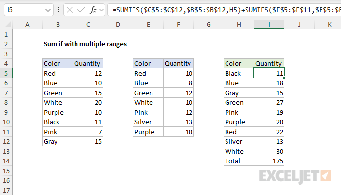
Notice that we have carefully locked the sum_range and criteria_range in each SUMIFS formula so that these don't change as the formula is copied down the table. The criteria (H5) is a relative address because we want this to change. The values in the range H5:H14 have been entered manually. The last formula in cell I14 uses the SUM function to sum all results:
=SUM(I5:I13)
This approach works fine, but it requires a fair bit of manual effort to set things up. If colors are added, we'll need to update the manual list in column H. Worse, as we add more ranges, the formula will become more and more complicated. How can we avoid this problem? In the latest version of Excel, the VSTACK function provides a nice way to simplify things.
Note: One way to make things easier would be to define each range as an Excel Table. This would allow us to use structured references instead of absolute references and make the formula easier to enter and read. Plus, using Excel Tables would make each range dynamic so that they will expand to include new data. However, we would still need to keep the color list in sync manually and add another SUMIFS function to the formula each time we add a new range.
Using the VSTACK function
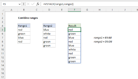
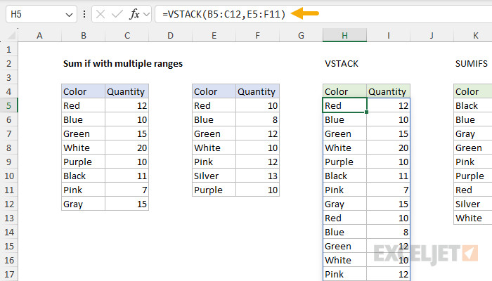
The VSTACK function combines multiple ranges into one range by stacking each new range below the first range. We can use VSTACK to help simplify this problem by first combining the two ranges, then using just one SUMIFS function to calculate a total for each color. You can see this approach in the screen below. The formula in H5 combines the ranges with VSTACK like this:
=VSTACK(B5:C12,E5:F11)
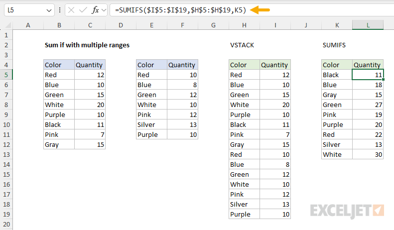
The formula in L5, copied down, uses SUMIFS just one time on the combined range:
=SUMIFS($I$5:$I$19,$H$5:$H$19,K5)
This works well and will scale nicely. For example, with three ranges, we can use VSTACK like this:
=VSTACK(range1,range2,range3)
VSTACK will combine all three ranges into one, and we can use SUMIFS on the combined range as before. However, we still need to maintain the colors listed in column K manually. How can we further streamline this process? The next logical step is to feed the result from VSTACK directly into a formula that will create all totals for us. We can do this by combining VSTACK with the GROUPBY function.
We can't feed the result from VSTACK directly into SUMIFS, unfortunately. Functions like SUMIFS, COUNTIFS, AVERAGEIFS, etc all require actual ranges for range arguments; you can't provide an array generated by another function.
Using VSTACK together with GROUPBY
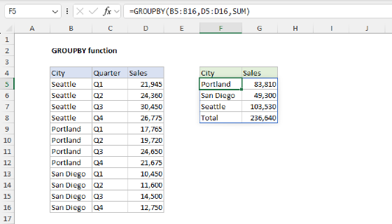
The GROUPBY function is designed to summarize data by grouping rows and aggregating values, a bit like a lightweight Pivot Table. In its simplest form, GROUPBY takes three arguments:
=GROUPBY(row_fields,values,function)
The row_fields argument contains the values for grouping data (the colors in this example). The values argument contains values that will be aggregated by the function specified (quantities in this example). Last, the function specifies the calculation to run (SUM in this case). To use GROUPBY for this problem, we need to do three things:
- Combine the ranges into a single range
- Split the combined range into two columns
- Feed the two columns into GROUPBY separately
We can perform all 3 tasks in a single formula like this entered in cell H5 below:
=LET(
data,VSTACK(B5:C12,E5:F11),
GROUPBY(CHOOSECOLS(data,1),CHOOSECOLS(data,2),SUM)
)
At the outermost level, we use the LET function to define the variable "data" using VSTACK:
data,VSTACK(B5:C12,E5:F11)
This step combines the two ranges and assigns the result to data. We do this to make the formula efficient and easy to read. Next, we call the GROUPBY function to generate a sum for each color like this:
GROUPBY(CHOOSECOLS(data,1),CHOOSECOLS(data,2),SUM)
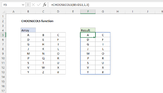
This is the one tricky step in the formula. We have already combined the ranges as data. However, GROUPBY needs the colors (row_fields) and quantities (values) separately, so inside GROUPBY, we use the CHOOSECOLS function to split data into two columns like this:
CHOOSECOLS(data,1) // colors
CHOOSECOLS(data,2) // quantities
The first column (colors) is fed into GROUPBY as the row_fields argument. The second column (quantities) is delivered as the values argument. Then, for the function argument, we provide SUM because we want to sum quantities by color. The final result is a table that lists all unique colors in the first column, and total quantities in the second column. This table is dynamic. If color names change, the table will automatically update. If we add more ranges to VSTACK, everything will continue to work properly. The result is similar to a Pivot Table, but there is no need to refresh the table manually.
Note: The Total row is created automatically. This can be disabled by setting total_depth to zero (0).
Key takeaways
- Conditional sums with multiple ranges is challenging because SUMIFS is designed to accept one range.
- SUMIFS can be adapted to sum multiple ranges, but it requires more manual configuration.
- VSTACK can combine non-contiguous ranges into one range to simplify calculations.
- GROUPBY can create summaries similar to pivot tables without manual refreshing.