Combine ranges

In this example, the goal is to combine ranges. With the introduction of the VSTACK function and the HSTACK function, this is quite a simple task. To combine ranges vertically, stacking one range on top of another, you can use the VSTACK function like this:

=VSTACK(range1,range2)

To combine ranges horizontally, you can use the HSTACK function like this:

=HSTACK(range1,range2)

In both formulas above, range1 (B5:B8) and range2 (D5:D9) are named ranges. The named ranges are for convenience only, you can use the raw cell references with the same result. For details on how these functions work see our documentation here: VSTACK function, HSTACK function.

Manual approach

Before the VSTACK and HSTACK functions where introduced, but after dynamic array formulas were available, it was possible to combine ranges with a more complex formula using the SEQUENCE function together with the LET function, the INDEX function, and the IF function. This is a much more manual approach, but it is an interesting example of how you can iterate through cells in a range keeping track of where you are as you go. The original formulas are below for reference. They are still useful for understanding how you can manipulate arrays in a formula.

Single column ranges

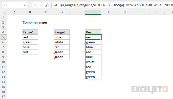
The formula to combine single column ranges is based on INDEX function, the SEQUENCE function, the IF function, and the LET function. In the example above, the formula in cell F5 is:

=LET(a,range1,b,range2,s,SEQUENCE(ROWS(a)+ROWS(b)),IF(s>ROWS(a),INDEX(b,s-ROWS(a)),INDEX(a,s)))

Adding line breaks to make the formula more readable, we have:

=LET(
   a,range1,
   b,range2,
   s,SEQUENCE(ROWS(a)+ROWS(b)),
   IF(s>ROWS(a),
      INDEX(b,s-ROWS(a)),
      INDEX(a,s)))

where range1 (B5:B8) and range2 (D5:D9) are named ranges. The first two lines inside let assign range1 to the variable "a" and assign range2 to the variable "b".

Note: Range1 and Range2 do not have to be provided as named ranges; you could instead use B5:B8 and D5:D9.

Next, the SEQUENCE function creates a numeric "row index" to cover all rows in both ranges:

=SEQUENCE(ROWS(a)+ROWS(b))
=SEQUENCE(9)
={1;2;3;4;5;6;7;8;9}

The resulting array is assigned to the variable "s". In the next line, the IF function is used to iterate through the array. If the current value s is greater than the rows in a, the INDEX function returns the value of b at row s minus the row count of a:

INDEX(b,s-ROWS(a)) // value from b

Otherwise, the INDEX function returns the value of a at row s:

INDEX(a,s) // value from a

The resulting values spill into the range F5:F13.

Note: a reader mentioned this formula to me based on the stackoverflow answer here.

Multiple column ranges

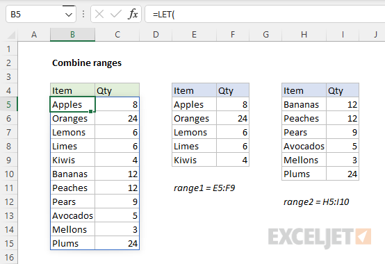
The formula to combine ranges with multiple columns is more complex. In the worksheet below, the formula in B5 looks like this

=LET(
   a,range1,
   b,range2,
   r,SEQUENCE(ROWS(a)+ROWS(b)),
   c,SEQUENCE(1,COLUMNS(a)),
   IF(
      r<=ROWS(a),
      INDEX(a,r,c),
      INDEX(b,r-ROWS(a),c))
)

where range1 (E5:F9) and range2 (H5:I10) are named ranges. Note that line breaks have been added for readability. 

Like the formula above, this formula figures out how many rows are in both ranges, and uses the SEQUENCE function to create a "row index" with the SEQUENCE function here:

SEQUENCE(ROWS(a)+ROWS(b)) // returns {1;2;3;4;5;6;7;8;9;10;11}

In a similar way, SEQUENCE is also used to create a "column index", named "c":

SEQUENCE(1,COLUMNS(a)) // returns {1,2}

The IF function tests all values in the row index sequence with the row count for range 1. When a row index value is less than or equal to the count of the rows in a (5), the INDEX function is used to fetch a row from range a at the current index value (r):

INDEX(a,r,c) // from range a

When a row index value is greater than 5, INDEX is used to fetch rows from b:

INDEX(b,r-ROWS(a),c))

Note c remains constant as {1,2} , the column index for range a. This is a shortcut to keep things simple. This formula does not try to figure out if the column counts for both ranges are the same or not. It simply assumes the column counts are the same and requests both columns.

Custom function with LAMBDA

The LAMBDA function can be used to create custom functions. The formula on this page is a good candidate, because it is relatively complex. When converted to a custom LAMBDA function, it is much easier to call:

=AppendRange(range1,range2)

See this article for more detail.