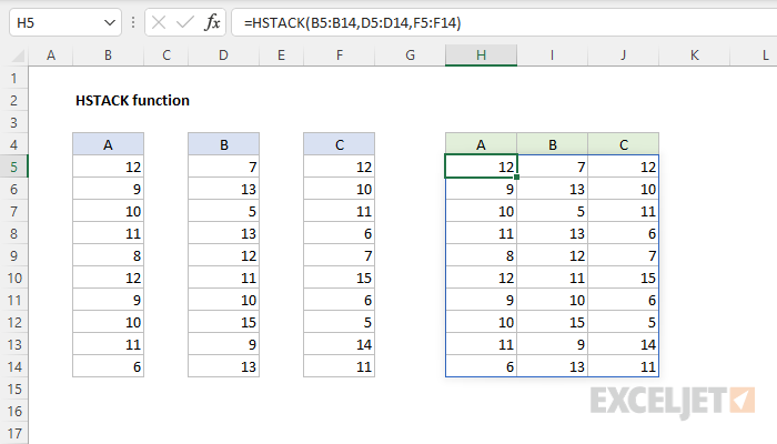
HSTACK Function

The HSTACK function combines arrays horizontally into a single array. Each subsequent array is appended to the right of the previous array. The result from HSTACK is a single array that spills onto the worksheet into multiple cells.

HSTACK works equally well for ranges on a worksheet or in-memory arrays created by a formula. The output from HSTACK is fully dynamic. If data in any given array changes, the result from HSTACK will update immediately. 

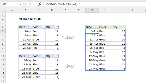
Use HSTACK to combine ranges horizontally and VSTACK to combine ranges vertically.

Basic usage

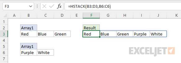
HSTACK stacks ranges or arrays horizontally. In the example below, the range B3:D3 is combined with the range B6:C6. Each subsequent range/array is appended to the right of the previous range/array. The formula in F3 is:

=HSTACK(B3:D3,B6:C6)

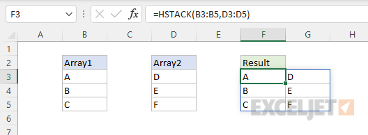
Ranges may include multiple rows, as seen below. The formula in F3 is:

=HSTACK(B3:B5,D3:D5)

Range with array

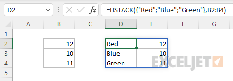
HSTACK can work interchangeably with both arrays and ranges. In the worksheet below, we combine the array constant {"Red";"Blue";"Green"} with the range B2:B4. The formula in F3 is:

=HSTACK({"Red";"Blue";"Green"},B2:B4)

Arrays of different sizes

When HSTACK is used with arrays of different sizes, the smaller array will be expanded to match the size of the larger array. In other words, the smaller array is "padded" to match the size of the larger array, as seen in the example below. The formula in cell F5 is:

=HSTACK(B5:B8,D5:D6)

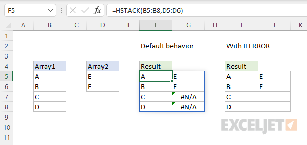
By default, the cells used for padding will display the #N/A error. One option for trapping these errors is to use the IFERROR function. The formula in I5 is:

=IFERROR(HSTACK(B5:B8,D5:D6),"")

In this formula, IFERROR is configured to replace errors with an empty string (""), which displays as an empty cell.