Summary
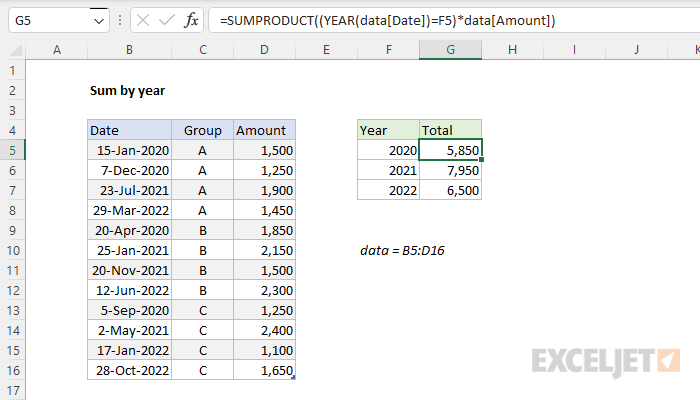
To sum values by year, you can use a formula based on the SUMPRODUCT function together with the YEAR function. In the example shown, the formula in cell G5 is:
=SUMPRODUCT((YEAR(data[Date])=F5)*data[Amount])
where data is an Excel Table in the range B5:D16. As the formula is copied down, it returns a total for each year shown in column F.
Generic formula
=SUMPRODUCT((YEAR(dates)=A1)*amounts)
Explanation
In this example, the goal is to calculate a total for each year that appears in column F. All data is in an Excel Table called data in the range B5:D16. The main challenge is that we have dates in column B, but we don't have separate year values to work with. The simplest way to solve this problem is with the SUMPRODUCT function using the formula seen in the worksheet above. The problem can also be solved with the SUMIFS function, or with a dynamic array formula. All three approaches are explained below.
SUMPRODUCT function
In the example shown, the formula in cell G5 is:
=SUMPRODUCT((YEAR(data[Date])=F5)*data[Amount])
Working from the inside out, the first step is to extract year values from the dates in column B, which is done with the YEAR function:
YEAR(data[Date]) // get years
Because there are 12 dates in the column, YEAR returns 12 results in an array like this:
{2020;2020;2021;2022;2020;2021;2021;2022;2020;2021;2022;2022}
Each year in this array corresponds to a date in data[Date]. Next, the year values are compared to the year in cell F5:
YEAR(data[Date])=F5
The result is an array of 12 TRUE and FALSE values like this:
{TRUE;TRUE;FALSE;FALSE;TRUE;FALSE;FALSE;FALSE;TRUE;FALSE;FALSE;FALSE}
Notice TRUE values correspond to dates that occur in 2020, the value in F5. Next, this array is multiplied by the amounts in column D. The math operation automatically converts the TRUE and FALSE values to 1s and 0s, so we can visualize this operation like this:
{1;1;0;0;1;0;0;0;1;0;0;0}*data[Amount]
Remember the 1s in the first array correspond to dates that occur in 2020, while 0s indicate dates in other years. The zeros in the first array effectively "cancel out" amounts in other years. The resulting array is returned to SUMPRODUCT like this:
=SUMPRODUCT({1500;1250;0;0;1850;0;0;0;1250;0;0;0})
With only one array to process, SUMPRODUCT sums the array and returns a final result of 5850. As the formula is copied down, the cell reference F5, which is relative, changes at each new row, and we get the correct total for each year shown.
Note: in the current version of Excel, you can replace the SUMPRODUCT function with the SUM function in the formula above. To read more about this topic, see Why SUMPRODUCT?
SUMIFS function
Another way to solve this problem is with the SUMIFS function and a formula like this:
=SUMIFS(data[Amount],data[Date],">="&DATE(F5,1,1),data[Date],"<="&DATE(F5,12,31))
If you are new to SUMIFS, this article covers the basics. This formula is more complicated than the SUMPRODUCT option because SUMIFS has no way to get at the year values directly. This limitation is discussed in more detail here. Instead, we need to create two dates for each year with the DATE function, then test for dates between these two dates:
DATE(F5,1,1) // start "Jan 1, 2020"
DATE(F5,12,31) // end "Dec 31,2020"
For the start date, we simply hardcode 1 for month and day arguments to get a January 1 date. For the end date, we hardcode 12 for month and 31 for day to create a December 31 date. For both dates, year comes from cell F5, which contains 2020. In summary, we use the DATE function to create a first-of-year date and a last-of-year date based on the year value in column F.
We also need logical operators to "bracket" each year. We concatenate the operators like this:
">="&DATE(F5,1,1) // start date
"<="&DATE(F5,12,31) // end date
The requirement to concatenate operators like this is again a "feature" of the SUMIFS function, which shares this peculiar syntax with eight other functions.
After the DATE function is evaluated, and after concatenation is complete, we have:
=SUMIFS(data[Amount],data[Date],">=43831",data[Date],"<=44196")
The number 43831 is the Excel serial number date for January 1, 2020. The number 44196 is the serial number for December 31, 2020.
Note: with either of the two options above, you could use the UNIQUE function to fetch the unique years from the dates as an initial step, if you have a modern version of Excel.
Dynamic array solution
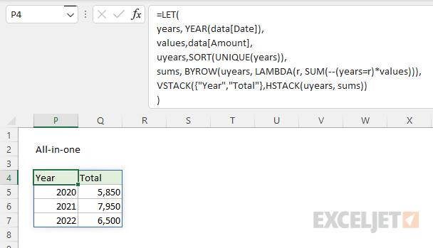
In the current version of Excel, which supports dynamic array formulas, it is possible to create a single all-in-one formula that builds the entire summary table, including headers, like this:
=LET(
years,YEAR(data[Date]),
values,data[Amount],
uyears,SORT(UNIQUE(years)),
sums, BYROW(uyears, LAMBDA(r, SUM(--(years=r)*values))),
VSTACK({"Year","Total"},HSTACK(uyears, sums))
)
Because this formula is doing a lot more work, it is more complicated. At the highest level, the LET function is used to assign values to four variables: years, values, uyears, and sums. First, we assign values to years and values like this:
=LET(
years,YEAR(data[Date]),
values,data[Amount],
Technically, we could just use the references for data[Date] and data[Amount] throughout the formula,but defining these variables up front makes the formula more portable. With a different set of data, only these two references need to be changed and the formula will continue to work.
The value for years is created with the YEAR function like this:
years,YEAR(data[Date]) // extract years
YEAR extracts just the year from all dates in data[Date]. Because the table contains 12 rows, the result is an array with 12 year values like this:
{2020;2020;2021;2022;2020;2021;2021;2022;2020;2021;2022;2022}
Next, values is assigned like this:
values,data[Amount]
As mentioned above, we do this to avoid repeating the reference elsewhere in the formula. In the following line, the value for uyears (unique years) is created like this:
SORT(UNIQUE(years)) // get and sort unique years
From the12 year values, the UNIQUE function returns just 3 unique years:
{2020;2021;2022} // unique
This array is returned to the SORT function, which sorts the array in ascending order:
{2020;2021;2022} // sorted
Note: In this example, it happens that the unique years are already in ascending order, so the SORT function does not change the result from UNIQUE. However, using the SORT function ensures that year values will always appear in order when source data is not sorted.
Next, the BYROW function is used to create a value for sums for each year like this:
sums,BYROW(uyears,LAMBDA(r,SUM(--(years=r)*values))) // sums
This is the core calculation in the formula. BYROW runs through the uyears values row by row. At each row, it applies this calculation:
LAMBDA(r,SUM(--(years=r)*values))
The value for r is the year in the "current" row. Inside the SUM function, this value is compared to years. Since years contains all 12 years, the result is an array with 12 TRUE and FALSE results. The TRUE and FALSE values are converted to 1s and 0s with the double negative (--), and the resulting array is multiplied by values. The 0s in the first array effectively "cancel out" amounts not associated with the year of interest.
Note: technically, the double negative (--) isn't needed here, because the math operation of multiplication automatically converts the TRUE and FALSE values to 1s and 0s. However, the double negative does no harm, and arguably makes the formula easier to read by clearly signaling an operation that cancels out values.
Next, the SUM function then sums the resulting array, which represents the total sum of values in the current year. Since there are 3 unique years, the result from BYROW is an array with 3 sums like this:
{5850;7950;6500} // sums
Finally, the HSTACK and VSTACK functions are used to assemble a complete table:
VSTACK({"Year","Total"},HSTACK(uyears, sums))
At the top of the table, the array constant {"Year","Total"} creates a header row. The HSTACK function combines uyears and sums horizontally, and the VSTACK function combines the header row and the data to make the final table. The result spills into multiple cells on the worksheet: