Summary
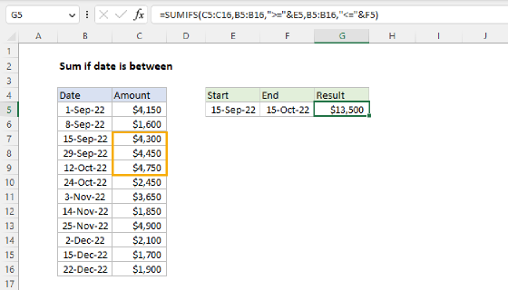
To sum values when corresponding dates are greater than a given date, you can use the SUMIFS function. In the example shown, the formula in cell G5 is:
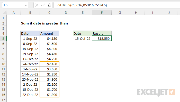
=SUMIFS(C5:C16,B5:B16,">"&E5)
The result is $18,550, the sum of Amounts in the range C5:C16 when the date in B5:B16 is greater than 15-Oct-2022.
Generic formula
=SUMIFS(values,dates,">="&A1)
Explanation
In this example, the goal is to sum amounts C5:C16 when the date in B5:B16 is greater than the date provided in cell E5. A good way to solve this problem is with the SUMIFS function.
Note: for SUMIFS to work correctly, the worksheet must use valid Excel dates. All dates in Excel have a numeric value underneath, and this is what allows SUMIFS to apply the logical criteria described below.
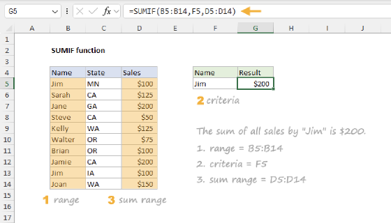
SUMIFS function
The SUMIFS function sums cells in a range that meet one or more conditions, referred to as criteria. The generic syntax for SUMIFS looks like this:
=SUMIFS(sum_range,range1,criteria1) // 1 condition
=SUMIFS(sum_range,range1,criteria1,range2,criteria2) // 2 conditions
In this problem, we need only one condition: the date in B5:B16 must be greater than the date provided in cell E5. To apply criteria, the SUMIFS function supports logical operators (>,<,<>,=) and wildcards (*,?) for partial matching. Each condition requires a separate range and criteria, and operators need to be enclosed in double quotes (""). We start off with the sum range, which contains the amounts in C5:C16:
=SUMIFS(C5:C16,
Next, we need to add criteria, which is provided in two parts. We add the range (B5:B16), then add the criteria (">="&E5):
=SUMIFS(C5:C16,B5:B16,">"&E5)
Notice we need to enclose the logical operator in double quotes (""), and join the text to the cell reference with concatenation. This is a quirk of the SUMIFS function. When we enter this formula, we get a sum of all amounts in C5:C16 where corresponding dates in B5B16 are greater than 15-Oct-2022, which is $18,550. Notice we are not including the start date in the result.
SUMIF function
Because this problem only requires a single condition, another option is to use the SUMIF function, an older function in Excel. The syntax is similar, but the order of the arguments is different. In the SUMIF function, the sum_range always comes last:
=SUMIF(B5:B16,">"&E5,C5:C16)
With hard-coded dates
In the example shown, the start date is exposed on the worksheet in cell E5. This is a nice solution, because it makes the start date easy to change. However, there may be times when you want to hardcode a date into a formula. In that case, the safest way to hardcode a date into the SUMIFS function is to use the DATE function, which generates a valid Excel date from the separate year, month, and day values. To sum amounts C5:C16 when the date in B5:B16 is greater than 15-Oct-2022, where the date is hardcoded, you can use a formula like this:
=SUMIFS(C5:C16,B5:B16,">"&DATE(2022,10,15))
Notice we still need to concatenate the logical operator ">" to the DATE function.