Summary
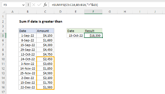
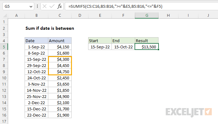
To sum values between a given start and end date, you can use the SUMIFS function. In the example shown, the formula in cell G5 is:
=SUMIFS(C5:C16,B5:B16,">="&E5,B5:B16,"<="&F5)
The result is $13,500, the sum of Amounts in the range C5:C16 when the date in B5:B16 is between 15-Sep-22 and 15-Oct-22, inclusive.
Generic formula
=SUMIFS(values,dates,">="&A1,dates,"<="&B1)
Explanation
In this example, the goal is to sum amounts in column C when the date in column B is between two given dates. The start date is provided in cell E5, and the end date is provided in cell F5. The date range should be inclusive - both the start date and end date should be included in the final result. A good way to solve this problem is with the SUMIFS function.
Note: for SUMIFS to work correctly, the worksheet must use valid Excel dates. All dates in Excel have a numeric value underneath, and this is what allows SUMIFS to apply the logical criteria described below.
SUMIFS with a date range
The generic syntax for using SUMIFS with a date range looks like this:
=SUMIFS(sum_range,criteria_range1,criteria1,criteria_range2,criteria2)
Where the arguments above have the following meaning:
- sum_range - the range that contains values to sum
- criteria_range1 - a range that contains the dates
- criteria1 - logic to target dates greater than the start date
- criteria_range2 - a range that contains the dates
- criteria2 - logic to target dates less than the end date
In the worksheet shown, we already have a start date entered in cell E5 (15-Sep-2022) and an end date in F5 (15-Oct-2022), so we will need to use those cell references as we enter criteria into SUMIFS. We start off with the sum range, which contains the amounts in C5:C16:
=SUMIFS(C5:C16,
Note that values in this range must be numeric. Next, we need to add the logic needed to target dates greater than or equal to the date in cell E5. We do this by entering two arguments: criteria_range1 and criteria1. We first add the range that contains the dates (B5:B16), then we add the criteria, which we enter as ">="&E5:
=SUMIFS(C5:C16,B5:B16,">="&E5,
This tricky syntax is a quirk of all the RACON functions in Excel. Notice that we need to enclose the operator in double quotes (">="), and concatenate the cell reference E5 with an ampersand (&). If we enter this formula as-is, we get a sum of all amounts in C5:C16 that are greater than or equal to 15-Sep-2022, which is $32,050:
=SUMIFS(C5:C16,B5:B16,">="&E5) // returns 32050
This is a valid result, but we aren't done yet, because we still need to add the second criteria for the end date in cell F5. We do this in the same way, by adding two more arguments: criteria_range2 and criteria2. We first add the date range (B5:B16):
=SUMIFS(C5:C16,B5:B16,">="&E5,B5:B16,
Then we add the criteria:
=SUMIFS(C5:C16,B5:B16,">="&E5,B5:B16,"<="&F5)
Notice we use the same date range (B5:B16) for criteria_range2 and, as before, we need to enclose the operator in double quotes ("<=") and concatenate cell F5 with an ampersand (&). When we enter the formula, SUMIFS returns $13,500, the total of Amounts in C5:C16 that are between 15-Sep-2022 and 15-Oct-2022, inclusive. If the dates in cell E5 or cell F5 are changed, the formula will immediately calculate a new result.
With hard-coded dates
In general, it is a best practice to enter the dates you want to use in a formula directly on the worksheet. This makes the worksheet more "transparent" because you can easily see the dates being used, and easily change the dates when needed. It also reduces the problem of Excel incorrectly interpreting a date, since you can see at a glance if dates on the worksheet are displayed correctly. That said, there may be times when you need to hardcode dates directly into a formula. The safest way to do this is to use the DATE function, which creates a valid date with separate year, month, and day arguments like this:
=DATE(year,month,day)
In this example, we can adapt the SUMIFS function above to use hardcoded dates by incorporating the DATE function inside the SUMIFS function like this:
=SUMIFS(C5:C16,B5:B16,">="&DATE(2022,9,15),B5:B16,"<="&DATE(2022,10,15))
- sum_range - C5:C16
- criteria_range1 - B5:B16
- criteria1 - ">="&DATE(2022,9,15)
- criteria_range2 - B5:B16
- criteria1 - "<="&DATE(2022,10,15)
Notice we still need to concatenate the logical operators to the DATE function using an ampersand (&).