Sum if cells are not equal to

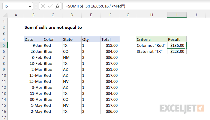
In this example the goal is to sum the numbers in the range F5:F16 when corresponding cells in the range C5:C15 are not equal to "Red". To solve this problem, you can use either the SUMIFS function or the SUMIF function. The SUMIF function is an older function that supports only one criteria. SUMIFS on the other hand can be configured to apply multiple criteria. Both options are explained below.

SUMIFS solution

In the example shown, the solution is based on the SUMIFS function. The formula in cell I5 is:

=SUMIFS(F5:F16,C5:C16,"<>red") // sum if not "red"

In this formula, sum_range is F5:F16, criteria_range1 is C5:C16, and criteria1 is "<>red". The result ($136) is the sum of numbers in the range F5:F16 when corresponding cells in C5:C15 are not "Red". Note that the SUMIFS function is not case-sensitive. With a criteria of "<>red", SUMIFS will exclude "RED", "Red", and "red". Also note that in the SUMIFS function, sum_range always comes first. To sum numbers when the state is not "TX" , you can adapt the formula like this:

=SUMIFS(F5:F16,D5:D16,"<>tx") // sum if not "tx"

In this formula, sum_range is F5:F16 as before, criteria_range1 is D5:D16, and criteria1 is "<>tx". For more information about using SUMIFS to apply multiple criteria with logical operators (>,<,<>,=) and wildcards (*,?), see this page.

SUMIF solution

The SUMIF function is an older function in Excel that supports only a single condition. To solve this problem with the SUMIF function, you can use a formula like this:

=SUMIF(C5:C16,"<>red",F5:F16)

In this formula, range is D5:D16, criteria is "<>tx", and sum_range is F5:F16. Note that in the SUMIF function, sum_range always comes last. The result ($136) is the same as with the SUMIFS function above. For more information about using SUMIF to apply criteria with logical operators (>,<,<>,=) and wildcards (*,?), see this page.

Notes

• For a case-sensitive solution, see this formula.
• To match a substring in a cell, see this formula.