Summary
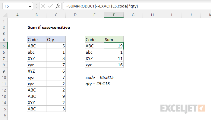
To calculate a case-sensitive "sum if", you can use a formula based on the EXACT function and the SUMPRODUCT function. In the example shown, the formula in F5, copied down, is:
=SUMPRODUCT(--EXACT(E5,code)*qty)
Where code (B5:B15) and qty (C5:C15) are named ranges. The result is a case-sensitive sum of quantities for each code listed in column E.
Generic formula
=SUMPRODUCT(--EXACT(A1,range1)*range2)
Explanation
In this example, the goal is to sum the quantities in column C by the codes in column E in a case-sensitive manner. The SUMIF function and the SUMIFS function are both good options for counting text values, and both functions support wildcards. However, neither function is case-sensitive, so they can't be used to solve this problem. A good solution is to use the EXACT function with the SUMPRODUCT function, as explained below.
Unique values
To generate the list of unique values in the range E5:E8, you would normally use the UNIQUE function. However, UNIQUE is not case-sensitive, so it will not work in this situation. This article provides a formula that can extract unique values from a range of cells, taking into account upper and lowercase characters.
EXACT function
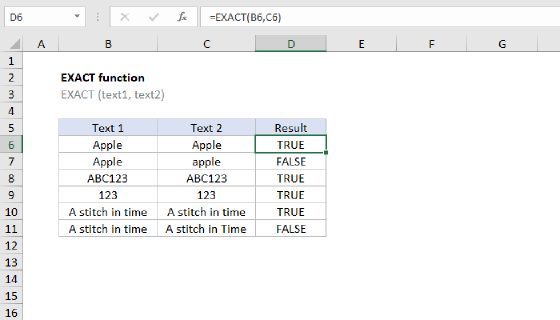
The EXACT function has just one purpose: to compare text in a case-sensitive manner. EXACT takes two arguments: text1 and text2. If text1 and text2 match exactly (considering upper and lower case), EXACT returns TRUE. Otherwise, EXACT returns FALSE:
=EXACT("abc","abc") // returns TRUE
=EXACT("abc","ABC") // returns FALSE
=EXACT("abc","Abc") // returns FALSE
=EXACT("ABC","ABC") // returns TRUE
Worksheet example
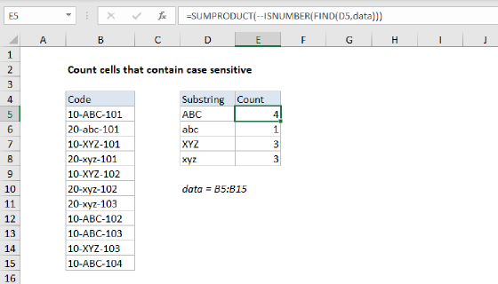
In the example shown, we have four codes in column E, and we want to sum the values in column C using the codes that appear in column B. In other words, we want to sum the total quantity per code, and this calculation needs to be case-sensitive. For convenience, code (B5:B15) and qty (C5:C15) are named ranges. The formula in E5, copied down, is:
=SUMPRODUCT(--EXACT(E5,code)*qty)
Working from the inside-out, we are using the EXACT function to compare each code in column E with the named range code (B5:B15):
--EXACT(E5,code)
EXACT compares the value in E5 ("ABC") to all values in B5:B15. Because the range contains 11 cells, EXACT returns 11 results (one for each code) in an array like this:
--{TRUE;FALSE;FALSE;FALSE;FALSE;FALSE;FALSE;TRUE;TRUE;FALSE;TRUE}
Each TRUE represents an exact match of "ABC" in B5:B15. Each FALSE represents a non-match. Next, we use a double-negative (--) operation to convert TRUE and FALSE values into 1's and 0's. The resulting array looks like this:
{1;0;0;0;0;0;0;1;1;0;1} // 11 results
Note: technically, the double negative (--) is unnecessary in this formula, because multiplying the TRUE and FALSE values by the numeric values in qty will automatically convert TRUE and FALSE values to 1s and 0s. However, the double negative does no harm, and it makes the formula a bit easier to understand, because it signals a Boolean operation.
At this point, we can simplify the formula like this:
=SUMPRODUCT({1;0;0;0;0;0;0;1;1;0;1}*qty)
Next, we need to perform the multiplication step and sum things up.
SUMPRODUCT function
SUMPRODUCT is a versatile function that appears in many formulas because it can handle array operations natively in older versions of Excel. In this case, the array operation is performed by the EXACT function in the previous step. The remaining steps look like this:
=SUMPRODUCT({1;0;0;0;0;0;0;1;1;0;1}*qty)
=SUMPRODUCT({1;0;0;0;0;0;0;1;1;0;1}*{5;1;3;7;6;7;2;2;9;2;3})
=SUMPRODUCT({5;0;0;0;0;0;0;2;9;0;3})
=19
As you can see, the array returned by EXACT behaves like a filter that "cancels out" values in qty that are not associated with the code "ABC". With just one array to process in the end, SUMPRODUCT sums all numbers in the array and returns the final result: 19. As the formula is copied down, we get the correct sum for each code in column E, taking into account upper and lower case characters.
Note: Because SUMPRODUCT can handle arrays natively, it is not necessary to use Control+Shift+Enter to enter this formula. In Excel 365, you can replace SUMPRODUCT with the SUM function. To read more about this, see Why SUMPRODUCT?