Summary
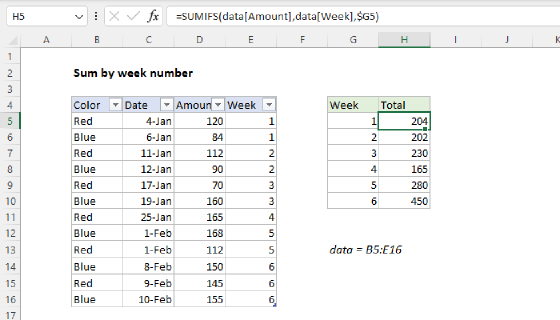
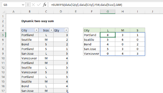
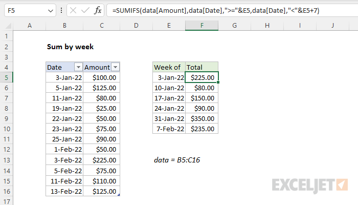
To sum values by week, you can use a formula based on the SUMIFS function. In the example shown, the formula in F5 is:
=SUMIFS(data[Amount],data[Date],">="&E5,data[Date],"<"&E5+7)
where data is an Excel Table in the range B5:C16, and the dates in E5:E10 are Mondays.
Generic formula
=SUMIFS(values,date,">="&A1,date,"<"&A1+7)
Explanation
In this example, the goal is to sum the amounts in column C by week, using the dates in the range E5:E10 which are all Mondays. All data is in an Excel Table named data in the range B5:C16. This problem can be solved in a straightforward way with the SUMIFS function. In the current version of Excel, which supports dynamic array formulas, you can also create an all-in-one formula that builds the entire summary table in one step. Both approaches are explained in detail below.
SUMIFS solution
The SUMIFS function can sum values in a range conditionally based on multiple criteria. The pattern of the SUMIFS function looks like this:
=SUMIFS(sum_range,range1,criteria1,range2,criteria2,...)
Notice the sum_range comes first, followed by range/criteria pairs. Each range/criteria pair of arguments represents another condition.
In this case, we need to configure SUMIFS to sum values by week using two criteria: one to match dates greater than or equal to the first day of the week, one to match dates less than the first day of the next week. We start off with the sum_range and the first condition:
=SUMIFS(data[Amount],data[Date],">="&E5
Note: because we are using an Excel Table to hold the data, we automatically get the structured references seen above. If you are new to structured references, see this short video: Introduction to structured references.
The sum_range is data[Amount], criteria_range1 is data[Date], and criteria1 is ">="&E5. Notice we need to concatenate the greater than or equal to operator (>=) to the reference E5. This is because SUMIFS is in a group of eight functions that split formula criteria into two parts.
Next, we need to add a second range/criteria pair of arguments to target dates through the last day of the week:
=SUMIFS(data[Amount],data[Date],">="&E5,data[Date],"<"&E5+7)
Here, criteria_range2 is again data[Date], and criteria2 is "<"&E5+7. Basically, we add 7 days to the date in E5 and use the less than operator (<) to catch all days prior to the next week. Again, we need to use concatenation to join the operator to the cell reference. The reason we can add 7 days to E5 with simple addition is because Excel Dates are just serial numbers.
The formula is now complete. As the formula is copied down column F, the SUMIFS formula will generate a sum for each week using the date in column F.
Week of dates
The dates in column E are Mondays. The first date in E5 (3-Jan-22) is hard-coded, and the rest of the dates are calculated with a simple formula:
=E5+7
At each new row, the formula returns the next Monday in the calendar.
Dynamic array solution
In the current version of Excel, which supports dynamic array formulas, it is possible to create a single all-in-one formula that builds out the entire summary table, including headers, in one step like this:
=LET(
dates,data[Date],
amounts,data[Amount],
weeks,dates-WEEKDAY(dates,3),
uweeks,UNIQUE(weeks),
totals,BYROW(uweeks,LAMBDA(r,SUM((weeks=r)*amounts))),
VSTACK({"Week of","Total"},HSTACK(uweeks,totals)))
Note: Currently, VSTACK and HSTACK are only available through the Beta channel of Office Insiders. The Office Insiders program is free to join in Excel 365.
The LET function is used to assign values to five variables: dates, amounts, weeks, uweeks, and totals. First, we assign values to dates and amounts like this:
=LET(
dates,data[Date],
amounts,data[Amount]
Technically, we could just use the references data[date] and data[Amount] throughout the formula,but defining these variables for these up front keeps all worksheet references at the top of the code where they can be easily changed. In other words, by editing just these two references, you can easily adapt the formula to work with a different data set.
Next, the value for weeks is created like this:
weeks,dates-WEEKDAY(dates,3)
Here the WEEKDAY function is used to calculate a "Monday of the week" for each date in data[Date]. This formula is explained in more detail here. Because the table contains 12 rows of data, the result is an array with 12 dates like this:
{44564;44564;44571;44578;44578;44578;44585;44592;44592;44592;44599;44599}
Excel dates are just large serial numbers, so these are the raw numbers that correspond to the dates seen in E5:E10, which are all Mondays.
In the next line we define uweeks (unique weeks) with the UNIQUE function like this:
uweeks,UNIQUE(weeks)
We do this because we only want one row per week in our final summary table. The UNIQUE function returns the 6 dates seen in E5:E10, which are all Mondays:
{44564;44571;44578;44585;44592;44599}
Note: you could sort the result from UNIQUE with the SORT function to ensure that weeks are in the correct order if needed.
We are now ready to calculate the total amounts for each week. We do this with the BYROW function which generates the sums and assigns the result to the variable totals like this:
totals,BYROW(uweeks,LAMBDA(r,SUM((weeks=r)*amounts)))
BYROW runs through the uweeks values row by row. At each row, it applies this calculation with the LAMBDA function:
LAMBDA(r,SUM((weeks=r)*amounts))
The value of r is the date in the "current" row of uweeks. Inside the SUM function, the r is compared to weeks. Since weeks contains 12 dates for all 12 rows, the result is an array with 12 TRUE and FALSE results. The TRUE and FALSE values are multiplied by amounts. This math operation automatically converts the TRUE and FALSE values to 1s and 0s, and the zeros effectively "cancel out" the values in weeks not equal to r. The SUM function then sums the resulting array. When BYROW is finished, we have an array with 6 weekly sums like this:
{225;80;150;90;350;235} // totals
This is the value assigned to the variable totals.
Finally the HSTACK and VSTACK functions are used to assemble a complete table:
VSTACK({"Week of","Total"},HSTACK(uweeks,totals))
At the top of the table, the array constant {"Week of","Total"} creates a header row. The HSTACK function combines uweeks and totals horizontally, and the VSTACK function combines the header row and result from HSTACK vertically to make the final table. The final result spills into multiple cells on the worksheet.
Pivot Table solution
A pivot table is an excellent solution when you need to summarize data by year, month, quarter, and so on. For a side-by-side comparison of formulas vs. pivot tables, see this video: Why pivot tables.