IMAGE Function

The IMAGE function is Excel's solution for adding images to a worksheet with a formula. IMAGE is similar in some ways to HTML's <img> tag, which is used to add images to an HTML page. Like the <img> tag, the IMAGE function allows you to set the image path and provide options for fit and size. IMAGE supports many file formats, including BMP, JPG, JPEG, GIF, TIFF, PNG, ICO, and WEBP. The images must be available online and reachable with the "https://" protocol. As long as the path is valid and accessible, IMAGE will fetch the image and bring a copy of it into a cell on the worksheet. You can use the IMAGE function to add images to things like employee lists, product information, games, and other data that includes images.

Of course, you can manually insert an image into a cell anytime, so why use IMAGE? I think the main use case for IMAGE is importing a larger number of images with a formula that calculates the path to each image automatically. It might not matter much for 10 images, but for 100 images or a thousand, this is a big upgrade. The article below explains how to use IMAGE step-by-step, moving from simple hardcoded paths to formulas that calculate the path to an image using other information on the worksheet. Download the worksheet (link at top) to follow along.

Table of Contents

• Simple Example
• Argument details
• Example - Source path only
• Example - Custom size
• Example - Formula to generate source path
• Example - Formula with Alt Text
• Image caching

Simple Example

In its simplest form, the IMAGE function requires just the path to an image:

=IMAGE(source)

For example, to retrieve an image of the Norwegian flag (which exists on this website as the file "flag_norway.png", you can use the IMAGE function like this:

=IMAGE("https://exceljet.net/sites/default/files/flag_norway.png")

Which will return an image like this:

The image is returned to the cell in which the formula resides. See below for examples.

Argument details

The IMAGE function takes a total of five arguments, but only the first argument, source, is required.

• source - The absolute path to an image on the internet. This path should be provided as an absolute URL like "https://somedomain.com/images/target_image.png". Required.
• alt_text - A text description of the image for accessibility. Optional.
• sizing - a setting to control how IMAGE should handle the image size. Optional, with 4 possible values:
  • 0 - Fit the image into the cell and maintain its aspect ratio. This is the default behavior.
  • 1 - Fill the cell with the image. This setting will distort the image as needed to fill the cell.
  • 2 - Maintain the original image size. This setting will respect the original image size even if the image needs to expand outside the cell boundary.
  • 3 - Custom image size. This setting tells IMAGE that a custom height and/or width will be provided.
• height - A custom height for the image in pixels. Optional.
• width - A custom width for the image in pixels. Optional.

Example - Source path only

IMAGE returns an image directly to a cell. In the worksheet below, you can see an example of using the IMAGE function to return six different country flags. The formula in cell D5 (copied down) is configured to retrieve the full image path from column C as the source argument for IMAGE like this:

=IMAGE(C5)

You can see how this works below, where the IMAGE function has returned flag images for six countries: Canada, the United States, Germany, the United Kingdom, Mexico, and France. Note that these images already exist on the Exceljet.net server at the location specified in column C.

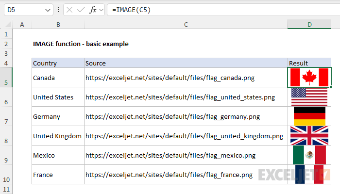
Note that the cell borders constrain the images. Essentially, the first edge to touch a cell boundary limits how far the image will expand. If you increase the row height or column width, you will see the image expand until it reaches its actual size.

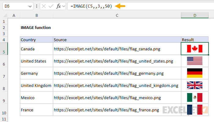
Example - Custom size

By default, the image will simply expand until it reaches the cell boundary, as seen above. However, it is possible to display the image at a custom size by setting the sizing argument to 3 and providing values for height and/or width. You can see how this works in the worksheet below, where we have configured IMAGE to set the width of each flag to 50 pixels:

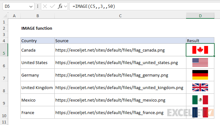
IMAGE is configured like this:

• source - C5 (the path in column C)
• alt_text - omitted
• sizing - 3 for custom size
• height - omitted
• width - 50 pixels

In addition to the configuration above, we have also set a custom alignment on all cells in the range D5:D10. Vertical alignment is set to "Middle", and Horizontal alignment is set to "Center". We have also set the row height to 30 (40 pixels). This creates the feeling of some white space padding around the flags. Note that sizing must be set to 3 before IMAGE will accept a custom height or width.

Example - Formula to generate source path

Because IMAGE accepts a path to an image as plain text, this text can be created programmatically with another formula. This is useful when the path to an image is predictable and can be constructed with other bits of information. In the worksheet example, all flag images follow the same pattern. They begin with "flag_" and end with the country name and a ".png" file extension:

flag_canada.png
flag_united_states.png
flag_germany.png
flag_united_kingdom.png
flag_mexico.png
flag_france.png

In addition, the path always begins with the same text:

"https://exceljet.net/sites/default/files/"

Because we already have the country names in column B, and because the flag images are consistently named, we have what we need to assemble each image path with a formula. This could be done in many ways, but in the worksheet below, we are using the SUBSTITUTE function together with the LOWER function in a formula like this:

=SUBSTITUTE("https://exceljet.net/sites/default/files/flag_xxxx.png",
"xxxx",SUBSTITUTE(LOWER(B5)," ","_"))

The main idea here is that we can start with the generic text slug:

"https://exceljet.net/sites/default/files/flag_xxxx.png"

And replace the placeholder "xxxx" with the country name we need. The complication is that we need to convert the country names to all lowercase and also replace spaces (" ") with underscores ("_"), which makes the formula more complex. You can see the result below, where the paths in column C are now created with the formula above:

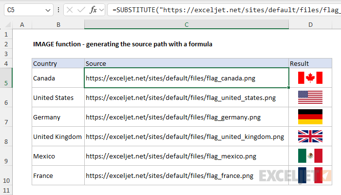
The formula in C5 works in three steps:

1. The LOWER function converts the country name in cell B5 to all lowercase and returns the result to the "inner" SUBSTITUTE function as the text argument.
2. The "inner" SUBSTITUTE function replaces all space characters (" ") with an underscore ("_") and returns the result to the "outer" SUBSTITUTE function as the new_text argument.
3. The "outer" SUBSTITUTE replaces the "xxxx" with the country name created in the two previous steps.

The IMAGE formula in cell D5 is the same as before:

=IMAGE(C5,,3,,50)

Example - Formula with Alt Text

Building on the example above, we can write a formula that includes a value for alt_text. In the worksheet below, we have moved the "template text" for the image path into cell C2 so that it is defined in just one place and removed the "Source" helper column. We have also added code to generate alt_text in the form of "Flag of Canada" for each flag image. The formula in cell C5 is:

=IMAGE(SUBSTITUTE($C$2,"xxxx",SUBSTITUTE(LOWER(B5)," ","_")),"Flag of "&B5,3,,50)

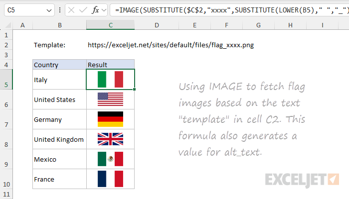
IMAGE is configured like this:

• source - SUBSTITUTE($C$2,"xxxx",SUBSTITUTE(LOWER(B5)," ","_"))
• alt_text - "Flag of "&B5
• sizing - 3 for custom size
• height - omitted
• width - 50 pixels

The source path is calculated as before by lowercasing the country name in column B, replacing spaces with underscores, and then replacing the "xxxx" in the template text with the result:

SUBSTITUTE($C$2,"xxxx",SUBSTITUTE(LOWER(B5)," ","_")) // source

The difference is that the text template comes from cell $C$2, which is supplied as an absolute reference to prevent changes when the formula is copied down. The alt_text is created by prepending "Flag of " to cell B5 with concatenation:

"Flag of "&B5 // alt_text

The result is the same as before but with a more compact and efficient formula that also adds alt text.

Note: As far as I know, you won't see the alt text anywhere except in the formula itself. However, you can convert the flag formulas to values like any other formula with Copy > Paste Special > Values. The result will leave the image and the alt text (visible in the formula bar) just like an image inserted manually with alt text added.

Image caching

One quirk of the IMAGE function is that it caches the images it fetches inside the worksheet. On the one hand, this is good because it means the images will display even without an internet connection. However, one consequence is that IMAGE holds on to cached images even when the source image as a destination path has changed. You would think that reentering the formula would cause IMAGE to reload an image from the source path, but I haven't seen this happen. Instead, it doggedly returns the old (cached) image. The only workaround I know is to delete the formula, save the workbook, and enter the formula again. If you know a better way, please let me know.

Notes

• IMAGE will only fetch images reachable at a path that begins with "https://".
• If an image is not found at the given path, IMAGE returns a #CONNECT error.
• If an image is at a redirected path, IMAGE returns a #CONNECT error.
• Sizing must be set to 3 before IMAGE will accept a custom height or width. Otherwise, IMAGE will return #VALUE!