Summary
This example shows how to create a mortgage payment schedule (also called a Mortgage Amortization Table) in Excel that includes extra payments. The schedule tracks interest, principal, extra payments, the total payment, and the remaining balance for each period. Two approaches are explained: (1) a single dynamic array formula that works in Excel 365, and (2) a traditional approach that works in older versions of Excel. Both solutions handle extra payments automatically, adjusting the schedule to show the loan paying off early when extra payments are applied. In addition to a recurring extra payment, both solutions support optional one-time payments that can be entered for any period. With the default assumptions in the workbook, which include an extra $500 payment each month, the loan is paid off in 240 months instead of 360, saving about $241,876 in interest.
Explanation
The goal of this example is to show how to create a mortgage payment schedule using Excel formulas. A mortgage payment schedule is a detailed breakdown of every payment over the life of a loan. Each payment represents one period, typically a month. For each period, the schedule shows how much of the payment goes toward interest, how much goes toward principal, and the remaining balance. The schedule also shows how early payments are mostly interest, while later payments shift toward principal.
This article walks through two approaches for building a payment schedule in Excel. The first is a single dynamic array formula that uses LET, SCAN, LAMBDA, FILTER, HSTACK, and VSTACK to generate the entire table at once. The second uses traditional formulas with named ranges that work in older versions of Excel. Both approaches include support for extra payments, including optional one-time payments for specific periods, so you can see exactly how additional principal payments shorten the loan term and reduce total interest.
This simplified example ignores property taxes, homeowner's insurance, mortgage insurance, and other fees.
In this article:
- Calculating a mortgage payment
- Key inputs and outputs
- Basic instructions
- Single formula solution
- Traditional formula solution
- Pros and cons
- Conclusion
Calculating a mortgage payment
The foundation of any payment schedule is the monthly payment itself. This is calculated with the PMT function, which returns the periodic payment for a loan given the interest rate, total number of payments, and loan amount:
=PMT(C5/12,C6*12,-C9)
The annual interest rate (C5) is divided by 12 to get a monthly rate, the term in years (C6) is multiplied by 12 to get total periods, and the loan amount (C9) is made negative because a loan represents a cash outflow. With the default assumptions (7% interest, 30-year term, $450,000 loan), PMT returns approximately $2,994 per month. For a more detailed walkthrough of this calculation, see estimate mortgage payment.
In a standard mortgage schedule without extra payments, Excel provides two handy functions for breaking down each payment. The IPMT function returns the interest portion, and the PPMT function returns the principal portion:
=IPMT(rate,per,nper,pv) // interest for a given period
=PPMT(rate,per,nper,pv) // principal for a given period
These functions work well when every payment is the same, because each period's interest and principal can be calculated independently. However, when extra payments are applied, the balance drops faster than the standard schedule assumes, and every subsequent interest calculation depends on the reduced balance from the previous period. Since IPMT and PPMT have no way to account for this, we need a different approach for each solution. The single formula version uses SCAN to track the running balance iteratively, and the traditional version calculates interest directly from the previous row's balance.
Key inputs and outputs
The key inputs and outputs appear in columns B and C:
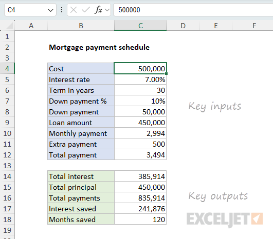
The inputs in column C drive both the payment schedule and the summary outputs. All values update dynamically when any input changes:
| Cell | Label | Value / Formula |
|---|---|---|
| C4 | Cost | 500000 |
| C5 | Interest rate | 7% |
| C6 | Term in years | 30 |
| C7 | Down payment % | 10% |
| C8 | Down payment | =C4*C7 |
| C9 | Loan amount | =C4-C8 |
| C10 | Monthly payment | =PMT(C5/12,C6*12,-C9) |
| C11 | Extra payment | 500 |
| C12 | Total payment | =C10+C11 |
The extra payment in C11 is the key input that makes this schedule different from a basic mortgage calculator. When set to zero, you get a standard payment schedule with no early payoff. When set to a positive value, both solutions automatically shorten the schedule and recalculate interest savings.
In addition to the recurring extra payment in C11, both solutions support optional one-time payments in column L. To make a one-time extra payment in a specific period, enter the amount in the corresponding row of column L. The one-time payment is added to the recurring extra payment for that period. When column L is empty, the schedule behaves exactly as before.
The outputs in C14:C18 summarize the overall impact of extra payments. In Sheet1 the formulas look like this:
| Cell | Label | Formula |
|---|---|---|
| C14 | Total interest | =SUM(INDEX(E5#,,2)) |
| C15 | Total principal | =SUM(INDEX(E5#,,3))+SUM(INDEX(E5#,,4)) |
| C16 | Total payments | =SUM(C14:C15) |
| C17 | Interest saved | =-CUMIPMT(C5/12,C612,C9,1,C612,0)-C14 |
| C18 | Months saved | =C6*12-MAX(INDEX(E5#,,1)) |
Note that some of these formulas use a spill range reference (E5#) with the INDEX function to reference specific columns in the spilled table. This syntax is specific to dynamic array formulas.
In Sheet2, the formulas look like this:
| Cell | Label | Formula |
|---|---|---|
| C14 | Total interest | =SUM(F:F) |
| C15 | Total principal | =SUM(G:G)+SUM(H:H) |
| C16 | Total payments | =SUM(C14:C15) |
| C17 | Interest saved | =-CUMIPMT(C5/12,C612,C9,1,C612,0)-C14 |
| C18 | Months saved | =C6*12-COUNTIF(I:I,">0") |
These formulas use full column references (e.g., F:F) instead of the spill range references in Sheet1.
Total interest (C14) sums the Interest column to get the total interest paid over the life of the loan. With the default assumptions, this is $385,914.
Total principal (C15) sums both the Principal and Extra Pmt columns. Together, these equal the original loan amount of $450,000.
Total payments (C16) adds total interest and total principal to get the grand total of all payments made: $835,914.
Interest saved (C17) uses the CUMIPMT function to calculate what total interest would have been over the full loan term without extra payments, then subtracts the actual total interest (C14). With the default assumptions, the $500 extra monthly payment saves $241,876 in interest.
Months saved (C18) subtracts the count of periods with a payment from the original number of periods. The result is 120 months - the loan is paid off 10 years early.
Both approaches use the same math. Given the same inputs, they should produce identical results. The workbook ships with the same assumptions in both sheets, so you can verify this for yourself. The two sheets work independently. If you change assumptions in one sheet, the mortgage table on that sheet will update accordingly, and the results will become out of sync with the other sheet.
Basic instructions
The purpose of this workbook is to explore how different variables affect the final term of a mortgage and the total amount paid as interest. By adjusting the inputs, you can quickly see how much money and time is saved with different scenarios:
- What if I add an extra $500 a month to my payment?
- What if I add one-time payments at certain times?
- What if I add/stop extra payments later?
The recurring extra payment in C11 and the one-time payments in column L make it easy to model these scenarios. One-time payments are especially useful for irregular income like bonuses, commissions, tax refunds, inheritance, or any situation where you have a lump sum to apply in a specific period.
To use the workbook, enter your loan details in cells C4:C7 and C11. Everything else updates automatically:
- Enter the home cost in C4. This is the total purchase price before the down payment.
- Enter the interest rate in C5 as a percentage (e.g., 7% or 0.07). This is the annual rate; the formulas convert it to a monthly rate internally.
- Enter the term in C6 as a number of years (e.g., 30).
- Enter the down payment percentage in C7 (e.g., 10% or 0.10). The down payment amount (C8) and loan amount (C9) are calculated automatically.
- Enter a recurring extra payment in C11. This amount is added to every monthly payment. Set it to zero for a standard schedule with no extra payments.
- Enter one-time payments in column L to model a lump-sum payment in a specific period. For example, to apply a $10,000 one-time payment in period 12, enter 10000 in cell L16 (row 16 corresponds to period 12 because the schedule starts in row 5). One-time payments are added on top of the recurring extra payment. Leave column L empty for no one-time payments.
The monthly payment (C10), total payment (C12), and the summary outputs in C14:C18 all recalculate when any input changes. The payment schedule in columns E:J updates as well — on Sheet1 the table resizes automatically, while on Sheet2 the formulas show zeros for periods after the loan is paid off.
If you're not sure which sheet to use, start with Sheet1 if you have Excel 365, or Sheet2 if you have an older version. Both produce the same results.
Single formula solution
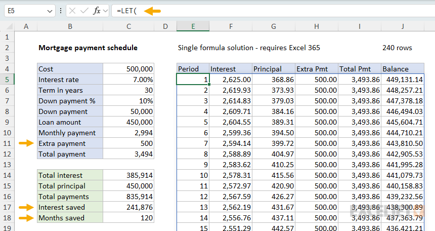
The single formula option requires Excel 365. The entire payment schedule is generated by a single dynamic array formula in cell E5:
=LET(
  loanAmt,C9,
  rate,C5/12,
  nper,C6*12,
  extraPmt,C11,
  pmt,PMT(rate,nper,-loanAmt),
  pers,SEQUENCE(nper),
  bals,SCAN(loanAmt,pers,LAMBDA(bal,per,
    LET(
      int,bal*rate,
      princ,IF(pmt-int<bal,pmt-int,bal),
      onetime,INDEX(L:L,4+per),
      extra,MIN(extraPmt+onetime,MAX(bal-princ,0)),
      MAX(bal-princ-extra,0)
    )
  )),
  prevBals,VSTACK(loanAmt,DROP(bals,-1)),
  onetimes,INDEX(L:L,4+pers),
  ints,prevBals*rate,
  princs,IF(pmt-ints<prevBals,pmt-ints,prevBals),
  extras,IF(extraPmt+onetimes<prevBals-princs,extraPmt+onetimes,prevBals-princs),
  totPmts,ints+princs+extras,
  result,FILTER(HSTACK(pers,ints,princs,extras,totPmts,bals),prevBals>0),
  result
)
The column headers in E4:J4 (Period, Interest, Principal, Extra Pmt, Total Pmt, Balance) are entered manually. The formula returns the data for all six columns, and the table grows or shrinks automatically when the inputs change.
Note: the original version of this formula (without extra payments) was suggested to me by Matt Hanchett, a reader of the Exceljet newsletter. It is a great example of how Excel's new dynamic array formula engine can be used to solve complicated problems with a single formula. Requires Excel 365 for now.
Variables in LET
The LET function defines named variables that make the formula easier to read and avoid repeated calculations. The first group sets up the core loan parameters:
- loanAmt - The loan amount (C9).
- rate - Monthly interest rate, calculated by dividing the annual rate (C5) by 12.
- nper - Total number of payment periods: term in years (C6) × 12.
- extraPmt - The extra monthly payment amount (C11).
- pmt - The standard monthly payment calculated by PMT.
- pers - A sequence of period numbers from 1 to nper, generated by SEQUENCE.
Calculating running balances with SCAN
The core of the formula is the bals variable, which uses SCAN with LAMBDA to iteratively calculate the remaining balance after each payment. Unlike a standard schedule, where you can use IPMT and PPMT to calculate each payment independently, extra payments change the balance in ways that depend on previous payments. SCAN is ideal for this kind of sequential calculation because it carries an accumulator value from one iteration to the next:
bals,SCAN(loanAmt,pers,LAMBDA(bal,per,
  LET(
    int,bal*rate,
    princ,IF(pmt-int<bal,pmt-int,bal),
    onetime,INDEX(L:L,4+per),
    extra,MIN(extraPmt+onetime,MAX(bal-princ,0)),
    MAX(bal-princ-extra,0)
  )
)),
SCAN starts with the loan amount as the initial accumulator value and loops through each period. At each step, the LAMBDA receives the current balance (bal) and calculates:
- int - Interest for the period: balance × monthly rate.
- princ - Principal portion of the regular payment: the lesser of (payment − interest) or the remaining balance, using IF to prevent overpayment.
- onetime - Any one-time payment for this period, looked up from column L using INDEX. The offset
4+permaps period 1 to row 5, period 2 to row 6, and so on, matching the schedule layout. - extra - The combined extra payment (recurring + one-time), capped at the remaining balance after principal with MIN.
- New balance - The remaining balance after subtracting principal and extra, floored to zero with the MAX function.
The result is an array of 360 balance values (one per period). Once the balance reaches zero, all subsequent values stay at zero.
Reconstructing payment details
Ideally, SCAN would return all columns (interest, principal, extra payment, and balance) in a single pass. However, Excel does not currently allow a formula to return an "array of arrays", so the formula uses a two-pass approach. In the first pass, SCAN calculates just the running balances. In the second pass, the formula reconstructs the other payment components from those balances.
The formula reconstructs the individual payment components as complete columns in the mortgage schedule. It first creates a prevBals array, which represents the balance at the start of each period, by prepending the original loan amount and dropping the last balance:
prevBals,VSTACK(loanAmt,DROP(bals,-1)),
VSTACK stacks the initial loan amount on top, and DROP removes the last value from bals so the arrays are the same size. From prevBals, the interest, principal, and extra payment are recalculated for each period:
onetimes,INDEX(L:L,4+pers),
ints,prevBals*rate,
princs,IF(pmt-ints<prevBals,pmt-ints,prevBals),
extras,IF(extraPmt+onetimes<prevBals-princs,extraPmt+onetimes,prevBals-princs),
totPmts,ints+princs+extras,
The onetimes variable uses INDEX to look up one-time payments from column L for all periods at once, using the same 4+pers offset as inside SCAN. These calculations mirror the logic inside SCAN but operate on the full arrays at once rather than through iteration. The pluralized names (ints, princs, extras, totPmts, onetimes) are a reminder that each variable holds a full column of values, in contrast to the singular variables (int, princ, extra, onetime) used inside the SCAN LAMBDA.
Note: I use INDEX above to get one-time payments instead of the OFFSET function. Although OFFSET would probably feel more natural to most people, it is a volatile function, so I generally avoid it when possible.
The overall structure of this formula is somewhat messy due to the two-pass approach. I also tested an alternative approach using REDUCE with VSTACK to build up the table row by row in a single pass. The result is a more readable formula, but it is pretty inefficient because VSTACK creates a new, larger array at every iteration. With 360 periods, this means Excel builds and discards hundreds of intermediate arrays. What we really need here is for Excel to support nested arrays, so that we can use SCAN in one pass to return the entire table.
Assembling the output with FILTER and HSTACK
Finally, HSTACK stacks the six columns side by side, and FILTER removes rows where the starting balance was already zero:
result,FILTER(HSTACK(pers,ints,princs,extras,totPmts,bals),prevBals>0),
result
FILTER is the reason the table automatically resizes. Extra payments reduce the total number of payments required, and once the balance is zero, all remaining payments are zero. FILTER hides these extra rows by allowing only rows with a balance greater than zero. With the default assumptions, only 240 of the 360 rows have a non-zero starting balance, so the formula returns exactly 240 rows. If you change the extra payment to zero, the table expands to 360 rows.
Conditional formatting for borders
Because the dynamic array formula controls how many rows appear in the schedule, cell borders can't be applied manually — the table might grow or shrink when the inputs change. Instead, two conditional formatting rules apply borders dynamically so they always match the current size of the schedule.
The first rule applies to the schedule area (E5:J1000) and uses the formula NOT(ISBLANK(E5)). This adds borders to every non-blank cell in the range, so borders appear only on rows that contain data from the spilled formula.
The second rule applies to the one-time payment column (L5:L1000) and uses the formula ROW(L5)<=MAX(E:E)+4. Since column L is not part of the spilled array, ISBLANK can't be used — the cells are empty by default. Instead, this rule checks whether the row falls within the active schedule by comparing the row number to the last period number. The +4 offset accounts for the fact that period 1 starts in row 5, so a schedule with 240 periods ends at row 244.
Note: I thought about combining the two rules into a single, more complex rule, but I decided to leave them separate since they illustrate different ways to format the "active" area of a worksheet.
Sheet2 does not use conditional formatting because the traditional approach requires manually copying formulas down, and cell formatting is copied along with the formulas.
Traditional formula solution
The traditional approach on Sheet2 uses individual formulas in each row and works in all versions of Excel. It uses four named ranges to keep the formulas readable:
| Name | Reference | Description |
|---|---|---|
| loan | C9 | Loan amount |
| rate | C5 | Annual interest rate |
| pmt | C10 | Monthly payment (from PMT) |
| extraPmt | C11 | Extra monthly payment |
First row formulas (row 5)
The first row of the schedule (period 1) uses the initial loan amount directly:
E5: 1
F5: =loan*rate/12
G5: =MIN(pmt-F5,loan)
H5: =MIN(extraPmt+L5,loan-G5)
I5: =F5+G5+H5
J5: =loan-G5-H5
Each formula calculates one column:
- Period (E5) - Hardcoded as 1.
- Interest (F5) - Loan amount × monthly interest rate.
- Principal (G5) - The standard payment minus interest, capped at the remaining balance with MIN to prevent overpayment on the final period.
- Extra payment (H5) - The recurring extra payment plus any one-time payment from column L, capped at the remaining balance after principal.
- Total payment (I5) - Sum of interest, principal, and extra.
- Balance (J5) - Previous balance minus principal and extra.
Subsequent row formulas (row 6 onward)
Starting in row 6, each formula references the balance from the previous row:
E6: =E5+1
F6: =J5*rate/12
G6: =MIN(pmt-F6,J5)
H6: =MIN(extraPmt+L6,J5-G6)
I6: =F6+G6+H6
J6: =J5-G6-H6
These formulas are copied down for 360 rows to handle a 30-year mortgage. The extra payment formula adds the recurring extra payment (C11) to any one-time payment in column L for that row. The use of MIN in the principal and extra payment columns prevents the principal from exceeding the remaining balance and ensures the extra payment doesn't push the balance below zero. When column L is empty, the cells evaluate to zero and the formula behaves exactly as before. Once the balance reaches zero in period 240, all subsequent rows show zeros for interest, principal, extra, and total payment.
Data validation
Since the traditional approach has a fixed number of rows (360), there is a danger that entering a longer term (like 50 years) will display incorrect results because the schedule is too short. The solution is to copy the formulas down to handle the full loan term. To warn the user in this situation, I've added data validation to cell C6 with a custom formula to prevent the term from exceeding the number of available rows:
=C6*12<=MAX(E:E)
If you enter a term greater than 30, the validation will warn the user that the schedule is "insufficient":
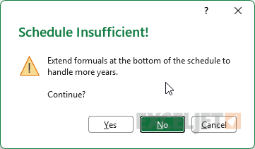
To resolve this warning and support a longer term, add more periods by copying the formulas in the last row into additional rows below. To support an additional 10 years, copy formulas into 120 additional rows. After adding rows, the data validation formula will automatically adjust since it references MAX(E:E), which picks up the new period numbers.
Pros and cons
Each approach has trade-offs worth considering. For the single formula solution in Sheet1, here are some pros and cons:
| Pros | Cons |
|---|---|
| Entire schedule in one formula | More complex, harder to debug |
| Auto-resizes when inputs change | Requires Excel 365 |
| No need to lock references or use named ranges | SCAN/LAMBDA can be intimidating |
| FILTER removes zero-balance rows automatically |
And here is a list of pros and cons for the traditional formula solution in Sheet2:
| Pros | Cons |
|---|---|
| Easier to understand and modify | Requires copying formulas down many rows |
| Easy to audit specific results | First row formulas are different |
| Works in all versions of Excel | Shows zero rows after payoff |
| Each column formula is independent | Needs named ranges for readability |
| Can handle up to 30 year term | Must copy formulas for longer terms |
Note that the named ranges in the traditional approach are not strictly required. You could replace loan with $C$9, rate with $C$5, and so on. However, the named ranges improve readability and eliminate the need to lock references with dollar signs when copying formulas down.
Conclusion
Extra payments can make a dramatic difference with a long-term mortgage. In this example, an extra $500 per month eliminates 10 years from a 30-year loan and saves over $241,000 in interest. This workbook makes it easy to explore different scenarios by changing the inputs in column C. You can also use the one-time payments in column L to model lump-sum scenarios (like applying a bonus, tax refund, or other windfall to a specific period) and immediately see the impact on total interest and loan term.
If you're using Excel 365, the single formula approach is elegant and self-adjusting. The table grows and shrinks dynamically as inputs change, and FILTER automatically removes rows where the loan has already been paid off. If you need to support older versions of Excel, the traditional approach with named ranges is straightforward and easier to audit. In both cases, the MIN logic ensures that the final payment is handled correctly, preventing the balance from going negative.
For more on the basics of calculating a mortgage payment, see estimate mortgage payment. For a deeper look at the functions used in the single formula, see the pages for LET, SCAN, LAMBDA, FILTER, HSTACK, and VSTACK.