Summary
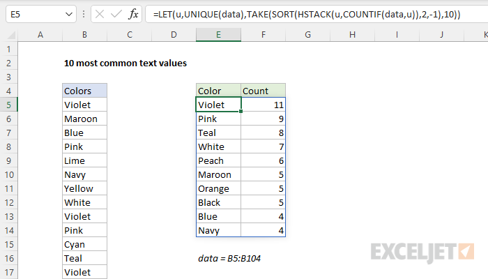
To list the 10 most common text values in a range, you can use a formula based on several functions, including UNIQUE, COUNTIF, SORT, and TAKE. In the example shown, the formula in cell E5 is:
=LET(u,UNIQUE(data),TAKE(SORT(HSTACK(u,COUNTIF(data,u)),2,-1),10))
Where data is the named range B5:B104. The result is the two-column table in E5:F14, with values sorted in descending order by count.
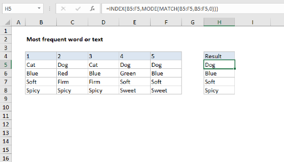
Note: This formula requires a current version of Excel. For Excel 2019 and older this formula will get the single most frequent text value. To list other frequently occurring values, a pivot table would be easiest.
Generic formula
=LET(u,UNIQUE(data),TAKE(SORT(HSTACK(u,COUNTIF(data,u)),2,-1),n))
Explanation
In this example, the goal is to list the 10 most frequently occurring text values in a range, in descending order by count, as seen in the range in E5:F14. This is an advanced formula that requires a number of nested functions. However, it is an excellent example of the power of dynamic array formulas in Excel. For convenience, data is the named range B5:B104. This range contains 100 random color names.
Get unique values
The first step in this problem is to get a list of unique colors from the data. This is easy to do with the UNIQUE function:
UNIQUE(data) // get unique colors
Since there 23 unique colors in B5:B104, UNIQUE returns an array containing 23 color names:
{"Violet";"Maroon";"Blue";"Pink";"Lime";"Navy";"Yellow";"White";"Cyan";"Teal";"Gold";"Orange";"Peach";"Black";"Turquoise";"Tan";"Red";"Green";"Gray";"Indigo";"Brown";"Purple";"Silver"}
Count unique values
Now that we have a list of values, the next step is to get a count for each unique value. This can be done with the COUNTIF function like this:
=COUNTIF(data,UNIQUE(data))
Here, the UNIQUE function returns the unique values in the data as the criteria argument, and COUNTIF calculates a count for each value. The result is an array with 23 counts like this:
{11;5;4;9;3;4;4;7;3;8;2;5;6;5;3;2;3;3;4;4;3;1;1}
We now have the basic ingredients we need to solve the problem.
Combine values and counts
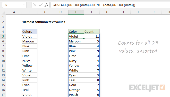
The next step is to combine the list of unique colors with the counts to form the two-column table seen in column E and F. This can be done with the HSTACK function, which is designed to combine arrays horizontally. We can use HSTACK like this:
=HSTACK(UNIQUE(data),COUNTIF(data,UNIQUE(data)))
The result from HSTACK is a list of 23 unique colors on the left, combined with 23 counts on the right:
We are getting close to a solution, but we still need to reorder the list to show the highest counts first, and drop all but the top 10 counts.
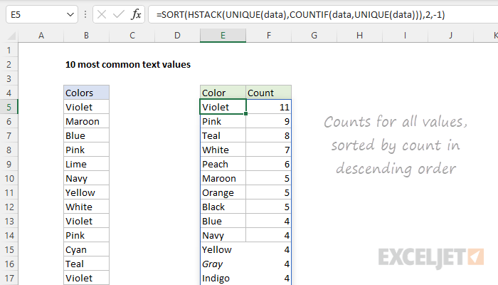
Sort by count
To sort the table by count, we can use the SORT function like this:
=SORT(HSTACK(UNIQUE(data),COUNTIF(data,UNIQUE(data))),2,-1)
Now we have the values sorted by count in descending order:
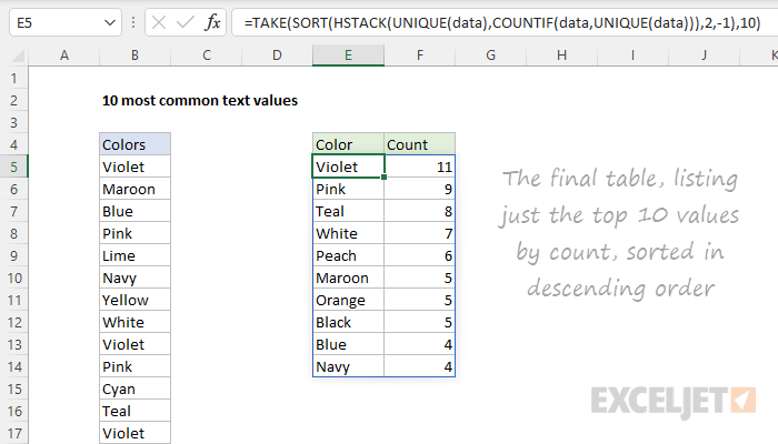
Top 10 values by count
The final step is to remove all but the top 10 values. The easiest way to do this is with the TAKE function, which is designed to extract rows and columns from arrays. In this case, we want the first 10 rows, so we provide 10 for rows:
=TAKE(SORT(HSTACK(UNIQUE(data),COUNTIF(data,UNIQUE(data))),2,-1),10)
The screen below shows the output of this formula:
Optimize
The formula above works fine, but it is a bit inefficient, since UNIQUE values are calculated twice. This might impact performance in larger sets of data. To streamline the formula, we can use the LET function. The LET function is used to declare and assign values to variables. In this case, we can use LET like this:
=LET(u,UNIQUE(data),TAKE(SORT(HSTACK(u,COUNTIF(data,u)),2,-1),10))
Here, we use UNIQUE to get unique values and assign the result to a variable named u. Then we replace UNIQUE(data) with u where it occurs in the formula. The result is that UNIQUE values are calculated just one time.