Pivot table most frequently occurring

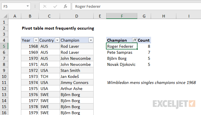
To list and count the most frequently occurring values in a set of data, you can use a pivot table.  In the example shown, the pivot table displays the top Wimbledon mens singles champions since 1968. The data itself does not have a count, so we use a pivot table to generate a count, then filter on this value. The result is a pivot table that shows the top 3 players, sorted in descending order by how often they appear in the list.

Note: When there are ties in top or bottom values, Excel will display all tied records.  In the example shown, the pivot table is filtered on top 3, but displays 4 players, because Borg and Djokovic are tied for third place.

Data

The source data contains three fields: Year, Country, and Champion. This data is contained in an Excel Table starting in cell B4. Excel Tables are dynamic and will automatically expand and contract as values are added or removed. This allows the Pivot Table to always show the latest list of unique values (after refresh).

Fields

In the pivot table itself, only the Champion field is used, once as a Row field, and once as a Value field (renamed "Count").

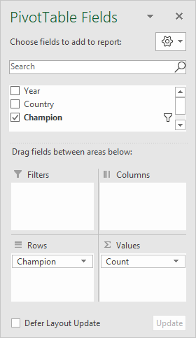
In the Values area, Champion is renamed "Count". Because Champion is a text field, the value is summarized by Sum.

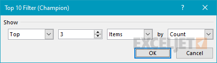
In the Rows area, the Champion field has a value filter applied, to show only the top 3 players by count (i.e. the number of times each player appears in the list):

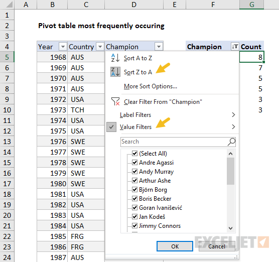
In addition, the Champions field is sorted by Count, largest to smallest:

Steps

1. Convert data to an Excel Table (optional)
2. Create a Pivot Table (Insert > Pivot Table)
3. Add the Champion field to the Rows area
   1. Rename to "Count"
   2. Filter on top 3 by count
   3. Sort largest to smallest (Z-A)
4. Disable Grand Totals for rows and columns
5. Change layout to Tabular (optional)
6. When data is updated, Refresh pivot Table for latest list