Sum if one of many things

To sum values when cells are equal to one of many things, you can use a formula based on the SUMIFS function and the SUMPRODUCT function. In the example shown, the formula in I5 is:

=SUMPRODUCT(SUMIFS(E5:E16,B5:B16,things))

where things is the named range G5:G7. The result is $19.50, the sum of Price where Item is "Apples", "Pears", or "Kiwis".

Explanation

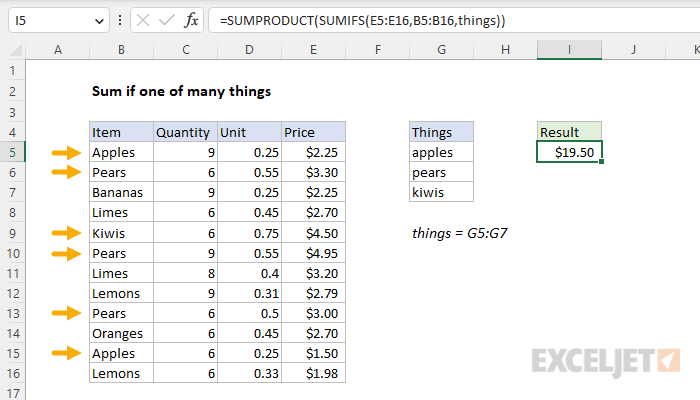
In this example, the goal is to sum the numbers in column E when the item in column B appears in the range G5:G7. The named range things is not required. It is used only for convenience and can be expanded as needed to include additional criteria. The article below explains several ways to solve this problem.

SUMIFS with SUMPRODUCT

One way to accomplish this is to give the SUMIFS function all three values in the named range things (G5:G7) as criteria, then use the SUMPRODUCT function to calculate a total. This is the approach in the worksheet shown, where the formula in I5 is:

=SUMPRODUCT(SUMIFS(E5:E16,B5:B16,things))

Working from the inside out, the SUMIFS function takes three arguments: sum_range, range, and criteria.

Sum_range is E5:E16 and contains the values we want to sum.
Range is B5:B15 and contains the values we are testing.
Criteria is the named range things (G5:G7), which contains 3 values.

When Excel evaluates this formula, it retrieves the values in things as an array like this:

=SUMPRODUCT(SUMIFS(E5:E16,B5:B16,{"apples";"pears";"kiwis"}))

Because SUMIFS receives 3 separate values for criteria, it returns 3 results in an array like this:

{3.75;11.25;4.5}

The first number is a sum for "apples", the second number is a sum for "Pears", and the last number is a sum for "Kiwis". These results are returned directly to the SUMPRODUCT function like this:

=SUMPRODUCT({3.75;11.25;4.5})

With just one array to process, SUMPRODUCT sums the array and returns a final result of $19.50.

Note: in the latest version of Excel, you can use the SUM function instead of SUMPRODUCT in this formula. Read more about this topic here: Why SUMPRODUCT?

ISNUMBER and MATCH

The above formula works fine, but has some limitations due to the nature of SUMIF. As an alternative, you can use the formula below, which uses the ISNUMBER function with the MATCH function to achieve the same result:

=SUMPRODUCT(--ISNUMBER(MATCH(B5:B16,things,0)),E5:E16)

This is a more flexible formula in cases where logical conditions become more complex. This formula shows one example.

FILTER function

This problem can also be solved in a more literal way with the FILTER function like this:

=SUM(FILTER(E5:E16,ISNUMBER(MATCH(B5:B16,things,0)),0))

In this formula, FILTER is configured to use ISNUMBER + MATCH to extract the Price of Items that appear in the named range things. The result is delivered to the SUM function which returns a final result. See this example for more details.