Explanation
In this example, the goal is to count the values in column B listed in the range E5:E7. One way to do this is to give the COUNTIF function all three values in the named range things (E5:E7) as criteria, then use the SUMPRODUCT function to get a total. The formula in G4 is:
=SUMPRODUCT(COUNTIF(B5:B15,things))
The COUNTIF function counts the number of cells in a range that meet criteria. When you give COUNTIF a range of cells as the criteria, it returns an array of numbers as the result, where each number represents the count of one thing in the criteria range. In this case, the named range things (D5:D7) contains 3 values, so COUNTIF returns 3 results in an array as shown below:
=COUNTIF(B5:B15,things)
=COUNTIF(B5:B15,{"apples";"pears";"kiwis"})
={2;3;1} // result from COUNTIF
Since "apple" appears twice, "pears" appears three times, and "kiwis" appears once, the array contains the numbers 2, 3, and 1. This array is returned directly to the SUMPRODUCT function:
=SUMPRODUCT({2;3;1})
With a single array to process, SUMPRODUCT simply sums the array and returns 6.
With an array constant
With a limited number of values, you can use an array constant in your formula like this:
=SUMPRODUCT(COUNTIF(B5:B15,{"apples","pears","kiwis"}))
ISNUMBER and MATCH
The above formula works fine, but has some limitations due to the nature of COUNTIF. As an alternative, you can use the formula below, which uses the ISNUMBER function with the MATCH function to achieve the same result:
=SUMPRODUCT(--ISNUMBER(MATCH(B5:B15,things,0)))
This is a more flexible formula in cases where logical conditions become more complex. It's also useful when you need to extract a value from a range in the data to use in a condition.


