ARRAYTOTEXT Function

The ARRAYTOTEXT function converts an array or range into a text string in a specific format that contains all values. Values are separated by commas (,) or semicolons (;), depending on the format requested and the structure of the array. ARRAYTOTEXT takes two arguments: array and format. Array is the array or range to convert to text. Array can be provided as a range like A1:A3 or an array generated by another function. The optional format argument controls the structure of the output. There are two formats available, concise and strict. The concise format is a simple, human-readable format. For example, values separated by commas. The strict format outputs a machine-parseable structure that describes an array in Excel. 

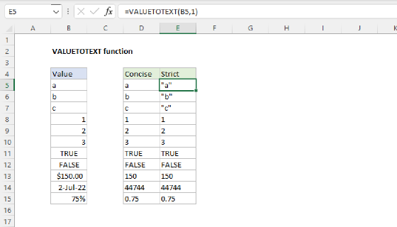
ARRAYTOTEXT is related to the VALUETOTEXT function, which performs the same kind of text conversion on single values.

Array syntax

All arrays in Excel are wrapped in curly brackets {}, and the delimiters between array elements indicate rows and/or columns. In the US version of Excel, a comma (,) separates columns and a semicolon (;) separates rows. For example, both arrays below contain numbers 1 through 3, but one is horizontal, and one is vertical:

{1,2,3} // columns (horizontal)
{1;2;3} // rows (vertical)

The array below shows the numbers 1-6 in three rows and two columns:

{1,2;3,4;5,6} // 3 rows x 2 columns

The commas (,) indicate a new column, and the semicolons (;) indicate a new row.

The delimiters used by the ARRAYTOTEXT function depend on the Regional settings for your computer. In the United States, the concise (default) format will always output a comma and a space (", ") between values.  When the format is set to strict, the delimiter between values in columns is a comma (","), and the delimiter between values in different rows is a semicolon (;). However, in other locales, the delimiter may vary. 

Concise format

When format is zero (0), ARRAYTOTEXT will return a concise format. Essentially, the concise format is a plain, human-readable text string separated by a comma and a space, regardless of the array's orientation. For example, if we have the values "Red", "Blue", and "Green" in the range A1:A3, the output from ARRAYTOTEXT looks like this:

=ARRAYTOTEXT(A1:A3) // returns "Red, Blue, Green"

If the values "Red", "Blue", and "Green" are in the range A1:C1 (i.e., columns instead of rows), the output is exactly the same:

=ARRAYTOTEXT(A1:C1) // returns "Red, Blue, Green"

In both cases, the delimiter is a comma followed by a space (", "), and the final text string contains no curly braces. ARRAYTOTEXT will output the concise format by default.

Because the concise format is a simple human-readable text string, you can sometimes use it as a shortcut in formulas that output delimited text strings (example here), as an alternative to the TEXTJOIN function. However, remember that ARRAYTOTEXT delimiters are based on regional settings, which vary by user. For example, if settings are for French/France, you will see semicolons (;) instead of commas. The other potential issue is that ARRAYTOTEXT has no control over empty values. TEXTJOIN is a better option if you need to control delimiters or ignore empty values. 

Strict format

When format is set to 1, ARRAYTOTEXT will return a text string that is a fully qualified array constant like {"red","blue","green"}. The output will appear wrapped in curly braces {}, and delimiters will follow the structure of the array provided — semicolons separating rows and commas separating columns in the US version of Excel. The strict format mirrors what you see in the formula bar if you enter a formula like this and use the keyboard shortcut F9:

=A1:C3

In fact, you can paste the strict output format directly into the formula bar, and Excel will return values to the worksheet in a range that follows the original structure of the array. For example, this formula will return a range with 6 cells (3 rows, and 2 columns):

={"red",1;"blue",2;"green",3}

You can use ARRAYTOTEXT with the strict format to get a fully qualified array constant that can be used inside another formula, just like a normal range or array. One potential use of ARRAYTOTEXT in strict mode is to store named values in a worksheet instead of named ranges. For example, suppose you have a small table, 5 rows x 3 columns, where the first column is alphabetic, and the other two are numeric.

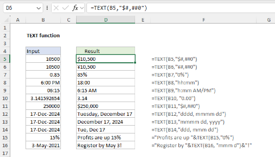
Note that ARRAYTOTEXT will always ignore number formatting, regardless of format.

Example - Basic usage

With the values 1, 2, and 3 in cells A1:A3, ARRAYTOTEXT returns the following in the default concise mode and in strict mode:

=ARRAYTOTEXT(A1:A3) // returns "1, 2, 3"
=ARRAYTOTEXT(A1:A3,1) // returns "{1;2;3}"

Notice that both results are text values, but in the second example, values are separated by semicolons, and the output is enclosed in curly braces. The strict format option will also wrap text values in double quotes (""). For example, with "red", "blue", and "green" in A1:A3:

=ARRAYTOTEXT(A1:A3) // returns "red, blue, green"
=ARRAYTOTEXT(A1:A3,1) // returns "{"red";"blue";"green"}"

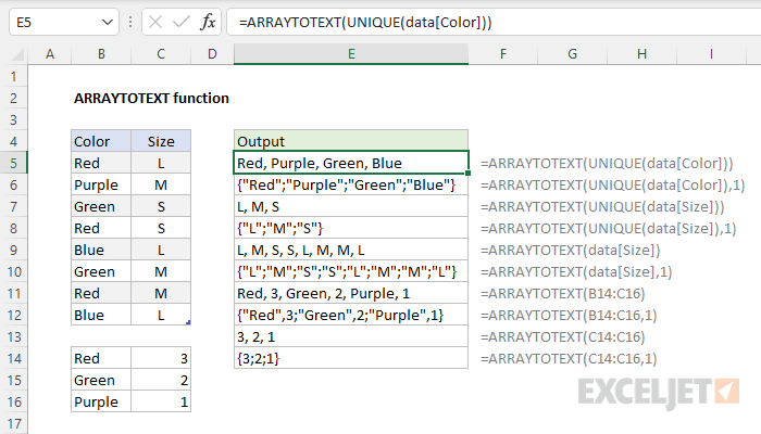
In the example shown above, the formula in E11 refers to a range that contains both text values and numbers:

=ARRAYTOTEXT(B14:C16) // returns "Red, 3, Green, 2, Purple, 1"
=ARRAYTOTEXT(B14:C16,1) // returns "{"Red",3;"Green",2;"Purple",1}"

Notice that only the second formula's text values are enclosed in double quotes. In addition, rows are separated by semicolons and columns are separated by commas, following the structure of arrays in the US version of Excel.

Example - Strict format to create a named value

Because ARRAYTOTEXT's strict format can create array constants, you can use it to create a named table. To give a table a name that you can refer to in a formula, without storing it as a range in the worksheet, you can follow a process like this:

1. Lay out the table in a worksheet
2. Invoke ARRAYTOTEXT on the table with strict format.
3. Copy the resulting value to the clipboard.
4. Open the name manager (Control + Shift + F3) and enter a name.
5. In "Refers to", type an equal sign (=) and paste the copied text.

You can now delete the original table in the workbook and use the name like an ordinary named range.

 Let me know if you discover another good use case for ARRAYTOTEXT.