Summary
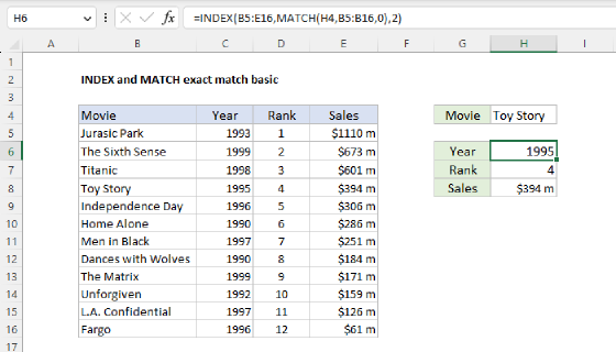
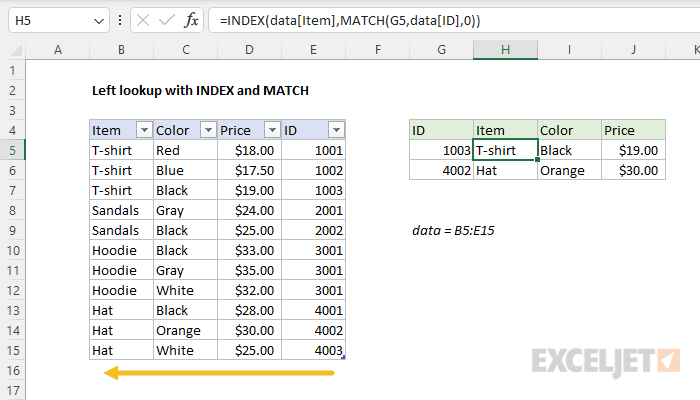
To perform a left lookup with INDEX and MATCH, set up the MATCH function to locate the lookup value in the column that contains lookup values. Then use the INDEX function to retrieve values at that position. In the example shown, the formula in H5 is:
=INDEX(data[Item],MATCH(G5,data[ID],0))
where data is an Excel Table in the range B5:E15.
Generic formula
=INDEX(range,MATCH(A1,range,0))
Explanation
In this example, the goal is to lookup data to the left of an ID that appears as the last column in the table. In other words, we need to locate a match in column E, then retrieve a value from a column to the left. This is one of those problems that is difficult with VLOOKUP, but easy with INDEX and MATCH or XLOOKUP. Both options are explained below.
Background study
- What is an Excel Table (3 min. video)
- Introduction to structured references (3 min. video)
- How to use INDEX and MATCH (overview)
- Excel Tables (overview)
INDEX and MATCH
One of the advantages of using INDEX and MATCH over VLOOKUP is that INDEX and MATCH can easily work with lookup values in any column of the data. In the example shown, columns B through E contain product data with a unique ID in column E. Using the ID in column G as a lookup value, the formulas in the range H5:J6 use INDEX and MATCH to retrieve the correct item, color, and price. In cell H5, the formula used to lookup Item is:
=INDEX(data[Item],MATCH(G5,data[ID],0))
Working from the inside out, the MATCH function is used to locate the value in G5 in the ID column like this:
MATCH(G5,data[ID],0) // returns 3
Here, the lookup_value is G5, the lookup_array is data[ID] (E5:E15), and match_type is set to zero for an exact match. The result from MATCH is 3, since the ID 1003 occurs in the third row of the table. This value is returned directly to the INDEX function as row_num. With array provided as data[Item], INDEX returns "T-shirt" as a final result:
=INDEX(item,3) // returns "T-shirt"
The same approach is used to retrieve the correct item, color, and price. The formulas in H5, I5, and J5 are as follows:
=INDEX(data[Item],MATCH(G5,data[ID],0)) // get item
=INDEX(data[Color],MATCH(G5,data[ID],0)) // get color
=INDEX(data[Price],MATCH(G5,data[ID],0)) // get price
Notice the MATCH function is used exactly the same way in each formula. The only difference is the array given to INDEX. Once MATCH returns 3 as a result for ID 1003, we have:
=INDEX(data[Item],3) // returns "T-shirt"
=INDEX(data[Color],3) // returns "Black"
=INDEX(data[Price],3) // returns 19
Each formula above returns the correct result for the ID 1003.
Locking references
The formulas above use normal references to make them easier to read. To lock references so that the same formula can be copied into the range H5:J6, we need to adjust the formula as follows:
=INDEX(data[Item],MATCH($G5,data[[ID]:[ID]],0))
Notice the reference to $G5 is now a mixed reference with the column locked. Also notice the reference to the ID column in the Excel Table data is also locked with the following syntax:
data[[ID]:[ID]] // locked
This syntax is unique to structured references, which are a feature of Excel Tables.
Video: How to copy and lock structured references
XLOOKUP function
The XLOOKUP function is a modern replacement of the VLOOKUP function. One of the features that VLOOKUP lacks, and XLOOKUP provides, is the ability to "look left" in a lookup operation. The equivalent XLOOKUP formulas to retrieve Item, Color, and Price are:
=XLOOKUP(G5,data[ID],data[Item]) // item
=XLOOKUP(G5,data[ID],data[Color]) // color
=XLOOKUP(G5,data[ID],data[Price]) // price
In these formulas lookup_value comes from G5, lookup_array is always data[ID], and return_array is the column from which to return data.
In addition, because XLOOKUP runs on the new dynamic array engine in Excel, you can retrieve values from all three columns at the same time like this:
=XLOOKUP(G5,data[ID],data[[Color]:[ID]])
This will cause XLOOKUP to return all three values at the same time as a spill range.