Summary
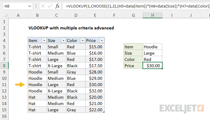
To apply multiple criteria with the VLOOKUP function you can use Boolean logic and the CHOOSE function. In the example shown, the formula in H8 is:
=VLOOKUP(1,CHOOSE({1,2},(H5=data[Item])*(H6=data[Size])*(H7=data[Color]),data[Price]),2,0)
where "data" is an Excel Table in B5:E15. The result is $30.00, the price of a Large Red Hoodie.
This is an array formula, and must be entered with control + shift + enter, except in Excel 365.
Explanation
In this example, the goal is to use VLOOKUP to retrieve the price for a given item based on three criteria: name, size, and color, which are entered in H5:H7. For example, for a Blue Medium T-shirt, VLOOKUP should return $16.00.
The VLOOKUP function does not handle multiple criteria natively. Normally VLOOKUP looks through the leftmost column in a table for a match, and returns a value from a given column in a matching row. There is no built-in way to supply multiple criteria.
This example works around this limitation by using Boolean logic to create an array of ones and zeros that represent rows that meet multiple conditions, then using this array to create a new table to provide to VLOOKUP. The overall process looks like this:
- Use Boolean logic to test Item, Size, and Color
- Create a new table with the CHOOSE function
- Provide the new table to VLOOKUP
- Configure VLOOKUP to look for 1 in the new table
This is a flexible way to apply multiple criteria with the VLOOKUP function. The logic can be extended as needed to apply more conditions, and each condition can use Excel's full range of formula logic.
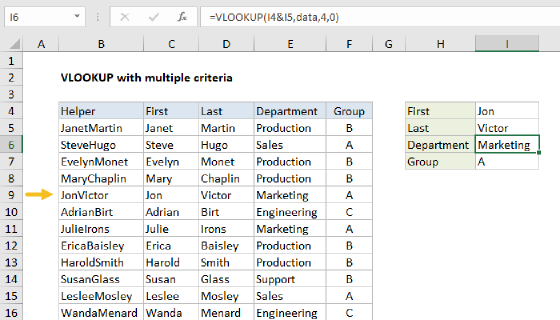
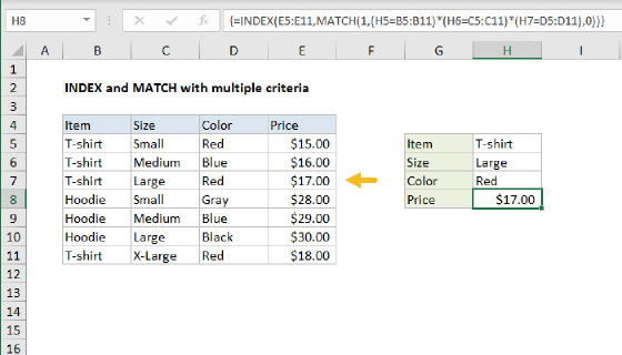
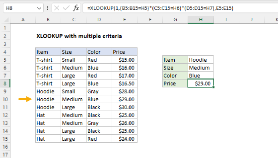
Note: This example shows an advanced technique to handle multiple criteria with VLOOKUP. If you have more basic needs, this formula takes a simple approach with a helper column. Other more flexible options include INDEX and MATCH and XLOOKUP.
Background study
This article assumes you are familiar with the VLOOKUP function and Excel Tables. If not, see:
- Excel Tables - introduction and overview
- VLOOKUP function - overview with examples
- Boolean algebra in Excel - 3 minute video
Boolean algebra for criteria
Working from the inside-out, the snippet below uses Boolean logic to create a temporary array of ones and zeros:
(H5=data[Item])*(H6=data[Size])*(H7=data[Color])
Here we compare the item in H5 against all items, the size in H6 against all sizes, and the color in H7 against all colors. The initial result is three arrays of TRUE/FALSE values like this:
={FALSE;FALSE;FALSE;FALSE;TRUE;TRUE;TRUE;TRUE;FALSE;FALSE;FALSE}*{FALSE;FALSE;TRUE;FALSE;FALSE;FALSE;TRUE;FALSE;FALSE;FALSE;TRUE}*{TRUE;FALSE;TRUE;FALSE;FALSE;FALSE;TRUE;FALSE;FALSE;TRUE;FALSE}
The math operation of multiplying the arrays together converts the TRUE FALSE values to 1s and 0s:
={0;0;0;0;1;1;1;1;0;0;0}*{0;0;1;0;0;0;1;0;0;0;1}*{1;0;1;0;0;0;1;0;0;1;0}
And after multiplication, we have a single array like this:
{0;0;0;0;0;0;1;0;0;0;0}
The process described above can be visualized as seen below. The "Result" array shows that the 7th row in the table meets all three conditions.
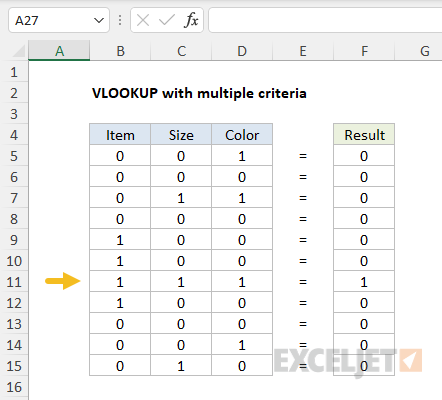
In the next step, we'll use the Result array to build a new table that we can use with VLOOKUP.
Creating a new table
We now have an array of TRUE and FALSE values that will work as a key to which row(s) in the table meet criteria. The problem is that this array is not actually part of the table VLOOKUP needs as the table_array argument. What we need is a new table, that combines the Result array from the Boolean operation above with the Price column of the table. We can do this with the CHOOSE function.
Normally, the CHOOSE function is used to select a value by numeric position. For example, to get the second value from a list of three values, you could use CHOOSE like this:
=CHOOSE(2,"red","blue","green") // returns "blue"
Notice the index_num argument is provided as 2 to get the second value. CHOOSE is flexible, and the values it accepts can be a mix of constants, cell references, arrays, and ranges. For this problem, we need to give CHOOSE two arrays: the Boolean result array, and the Price column of the table. Then, for index_num, we provide the array constant {1,2} like this:
CHOOSE({1,2},(H5=data[Item])*(H6=data[Size])*(H7=data[Color]),data[Price])
The array constant is the tricky part. By using {1,2} for index_num we are requesting the first and second value at the same time. The CHOOSE function dutifully complies, and returns both arrays "glued" together in a single array that looks like this:
{0,15;0,16;0,17;0,17.5;0,28;0,29;1,30;0,32;0,20;0,21;0,22}
In the above format, it is hard to see the structure of the array. However, if we place the array in an Excel worksheet, the structure becomes clear. As you can see, the array is a 2-column table:
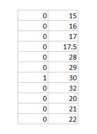
We now have a new table we can use in VLOOKUP.
VLOOKUP function
All of the work done so far has just one purpose: to create a new table that can be used in VLOOKUP as the table_array argument. Now we need to configure the VLOOKUP function. We start by providing a lookup value of 1, to match the structure of the new table:
=VLOOKUP(1
Next, we drop in the code explained above for table_array:
=VLOOKUP(1,CHOOSE({1,2},(H5=data[Item])*(H6=data[Size])*(H7=data[Color]),data[Price])
To wrap things up, we set col_index_num to 2, and range_lookup to 0. The final formula in H8 is:
=VLOOKUP(1,CHOOSE({1,2},(H5=data[Item])*(H6=data[Size])*(H7=data[Color]),data[Price]),2,0)
VLOOKUP matches the 1 in row 7, and returns 30 as a final result. If any of the input values in H5:H7 change, a new table is assembled and VLOOKUP returns a new result.
Note: This is an array formula, and must be entered with control + shift + enter, except in Excel 365.