SWITCH Function

The SWITCH function compares one value against a list of values and returns the result that corresponds to the first match. You can use SWITCH when you want a "self-contained" exact match lookup with several possible results, without a lookup table on the worksheet and without nesting multiple IF functions. If you have used a switch or case statement in a programming language, SWITCH works the same way: one value is checked against a list of cases, and the first case that matches decides the result.

The first argument in SWITCH is called expression, and it can be a hard-coded constant, a cell reference, or a formula that returns a value to match against. Matching values and their results follow as pairs, and SWITCH can handle up to 126 pairs. The last argument, default, is optional. When it is provided, SWITCH returns it if no match is found. When it is omitted and no match is found, SWITCH returns the #N/A error. SWITCH performs an exact match only, so you can't use logical operators like greater than (>) or less than (<) in the values. For conditions like that, see the IFS function, or the workaround in SWITCH with comparisons below.

The SWITCH function is available in Excel 2019 and later, including Excel 365. In older versions of Excel, use a nested IF function or a lookup function like VLOOKUP instead.

Key features

• Compares one expression against a list of values and returns the result paired with the first match
• Handles up to 126 value/result pairs in a single formula
• Performs exact matching only: not case-sensitive, no wildcards, no comparison operators
• Accepts an optional default value as the last argument
• Returns #N/A when no match is found and no default is provided
• The expression can be a value, a cell reference, or a formula
• Results can be text, numbers, or formulas
• Does not short-circuit; every value and result is evaluated

Table of contents

• Basic examples
• Translate codes to labels
• Return a default value
• Match the result of an expression
• A different calculation for each case
• SWITCH with comparisons
• SWITCH with arrays
• When a lookup table is better
• SWITCH and performance
• SWITCH versus IFS
• SWITCH versus CHOOSE
• Notes

Basic examples

A SWITCH formula with three value/result pairs and a default can be visualized like this:

=SWITCH(
expression, // value to match
value1,result1, // pair 1
value2,result2, // pair 2
value3,result3, // pair 3
default // optional
)

SWITCH compares expression to each value in turn and returns the result that follows the first matching value. For better readability, you can add line breaks to a SWITCH formula as shown above.

In the examples below, A1 contains the value to match. To translate a rating of 1, 2, or 3 into a label:

=SWITCH(A1,1,"Poor",2,"OK",3,"Good") // 2 returns "OK"
=SWITCH(A1,1,"Poor",2,"OK",3,"Good") // 4 returns #N/A
=SWITCH(A1,1,"Poor",2,"OK",3,"Good","?") // 4 returns "?"

The first formula returns "OK" for a rating of 2. The second formula is the same, but it returns #N/A for any rating other than 1, 2, or 3. The third formula adds a default value as the last argument, so an unrecognized rating returns "?" instead. SWITCH is not case-sensitive, so text values match regardless of case:

=SWITCH(A1,"S","Small","M","Medium","L","Large","Unknown") // "m" returns "Medium"

The expression can be a formula. To classify a date in A1 as a weekend or a weekday, you can match the number returned by the WEEKDAY function. By default, the WEEKDAY function returns 1 for Sunday and 7 for Saturday, so we need to test for 1 and 7 to determine a weekend:

=SWITCH(WEEKDAY(A1),1,"Weekend",7,"Weekend","Weekday") // 1 = Sunday, 7 = Saturday

Notice that "Weekend" appears twice. SWITCH has no way to assign one result to several values at once, so a shared result must be repeated for each value.

The equivalent formula with IF and OR looks like this:

=IF(OR(WEEKDAY(A1)=1,WEEKDAY(A1)=7),"Weekend","Weekday")

Translate codes to labels

A common use of SWITCH is to translate a code into a label. In the worksheet below, the goal is to convert the numeric rating in column C into a text result: 1 is "Poor", 2 is "OK", and 3 is "Good". Any other rating should return "?". The formula in D5, copied down, is:

=SWITCH(C5,1,"Poor",2,"OK",3,"Good","?")

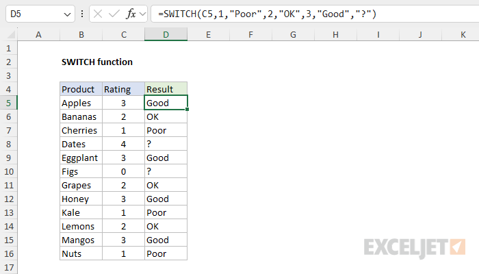
SWITCH compares the rating in C5 against three value/result pairs in order. A rating of 3 matches the third pair, so SWITCH returns "Good". The ratings 4 and 0 in C8 and C10 do not match any value, so SWITCH returns the default result, "?". Because the value being tested appears just once, at the start of the formula, a SWITCH formula is shorter and easier to read than the equivalent nested IF formula:

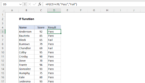
=IF(C5=1,"Poor",IF(C5=2,"OK",IF(C5=3,"Good","?")))

Or the equivalent IFS formula:

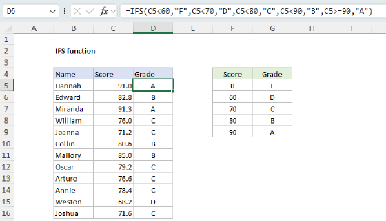
=IFS(C5=1,"Poor",C5=2,"OK",C5=3,"Good",TRUE,"?")

All three formulas return the same results. The nested IF version repeats the cell reference three times and needs three closing parentheses. The IFS version also repeats the cell reference in each test, and it needs TRUE as a final test to provide a default value. The SWITCH version reads as a simple list of values and results.

Return a default value

When SWITCH does not find a match, the result depends on whether a default value has been provided. In the worksheet below, the goal is to translate the size codes in column C into full names: "S" is "Small", "M" is "Medium", and "L" is "Large". The formula in D5, copied down, is:

=SWITCH(C5,"S","Small","M","Medium","L","Large")

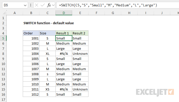
This works for the codes S, M, and L, but the codes "XL" in C8 and "XS" in C15 do not match any value, so SWITCH returns the #N/A error. To handle unrecognized codes, add a default value as the final argument. The formula in E5, copied down, is:

=SWITCH(C5,"S","Small","M","Medium","L","Large","Unknown")

Now the unrecognized codes return "Unknown" instead of #N/A. The default is simply the last argument, with no value to match. When the number of arguments after expression is odd, SWITCH treats the final argument as the default. Notice also that the lowercase "s" in C12 returns "Small", because SWITCH is not case-sensitive. If you want to return no result when there is no match, use an empty string ("") as the default.

The ability to easily set a default value is one subtle advantage SWITCH has over the IFS function, which requires a TRUE test as a workaround to provide a default.

Match the result of an expression

The first argument in SWITCH does not have to be a simple cell reference. It can be any formula that returns a value to match against. In the worksheet below, the goal is to classify each date in column B as a weekend or a weekday. The WEEKDAY function returns a number from 1 (Sunday) to 7 (Saturday), shown for reference in column C. The formula in D5, copied down, is:

=SWITCH(WEEKDAY(B5),1,"Weekend",7,"Weekend","Weekday")

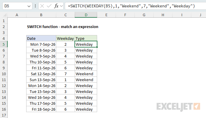
WEEKDAY runs first and returns a number, then SWITCH matches that number against the list. Saturday (7) and Sunday (1) both return "Weekend", and the default value returns "Weekday" for the other five days. Because SWITCH can only pair one value with one result, "Weekend" must be entered twice, once for each day. This is a limitation of SWITCH. When several values need to share a result and the list is long, the IFS function with the OR function or a lookup table is a better fit.

A different calculation for each case

The results in a SWITCH formula are not limited to constants. Each result can be a formula, which makes it possible to run a different calculation for each case. In the worksheet below, the goal is to convert all weights in column C to grams, based on the unit in column D. The formula in E5, copied down, is:

=SWITCH(D5,"kg",C5*1000,"g",C5,"lb",C5*453.6,"oz",C5*28.35)

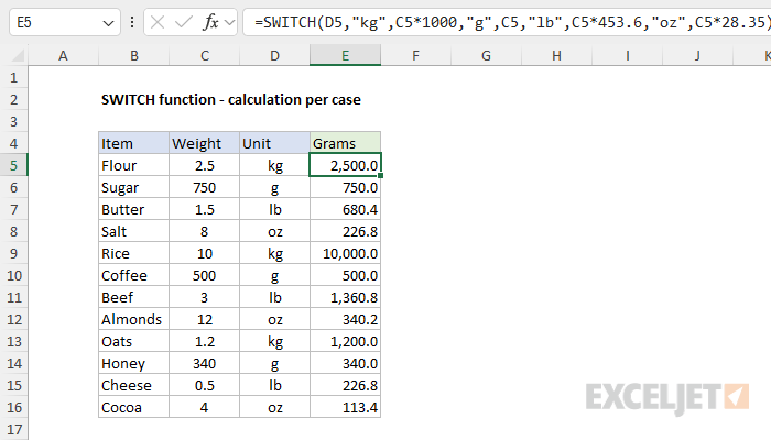
SWITCH matches the unit in D5 against four text values. For "kg", the result is the weight multiplied by 1000. For "g", the result is the weight as-is. For "lb" and "oz", the weight is multiplied by the number of grams in a pound and in an ounce. The result is a number, so it can be used directly in other calculations. There is no default value in this formula, so an unrecognized unit returns #N/A, which is a useful result when a conversion cannot be performed.

Be aware that Excel evaluates every result in a SWITCH formula, not just the one that is returned. This makes no practical difference for simple arithmetic, but it can affect performance when results involve slow calculations. See SWITCH and performance below.

SWITCH with comparisons

SWITCH performs exact matching only, so you can't use comparison operators like greater than (>) or less than (<) in the values. However, you can work around this limitation by using TRUE as the expression, and entering each value as a logical test. SWITCH then returns the result that follows the first test that evaluates to TRUE. In the worksheet below, the goal is to assign a tier to each customer based on sales in column C: 1,000 or more is "Gold", 500 or more is "Silver", and anything less is "Bronze". The formula in D5, copied down, is:

=SWITCH(TRUE,C5>=1000,"Gold",C5>=500,"Silver","Bronze")

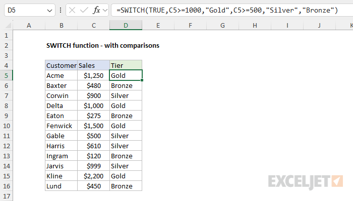
Each logical test returns TRUE or FALSE, and SWITCH compares these results to the expression, TRUE. For the sales value 900 in C7, the first test returns FALSE (900 is not 1,000 or greater), the second test returns TRUE, and SWITCH returns "Silver". The final argument, "Bronze", is the default, returned when no test is TRUE. As with any set of overlapping tests, the order matters: the tests must run from the highest threshold to the lowest, or the wrong tier will be returned.

This technique works, but it is really the IFS function structure written in a roundabout way. IFS is designed to take logical tests directly, so it is the more straightforward choice for conditions that involve comparisons:

=IFS(C5>=1000,"Gold",C5>=500,"Silver",TRUE,"Bronze")

See SWITCH versus IFS below.

SWITCH with arrays

In Excel 2021+ and Excel 365, the SWITCH function works with arrays. If the expression is a range or an array, SWITCH matches each value in the array separately and returns an array of results, which then spills onto the worksheet. This means a single SWITCH formula can translate an entire column of codes. In the worksheet below, the formula in D5 is:

=SWITCH(C5:C16,1,"Poor",2,"OK",3,"Good","?")

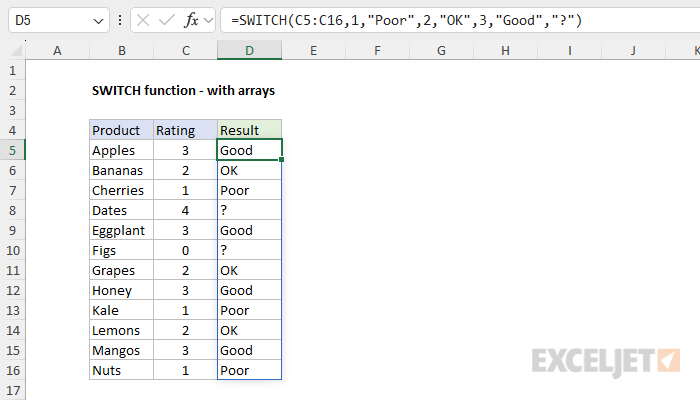
The formula is entered only in D5, and the results spill into D5:D16. The values and results are the same as in the first example above; the only change is that the expression is now the range C5:C16 instead of a single cell. Because the results spill, there is no need to copy the formula down, and the spill range will adjust automatically if the size of the input range changes.

Note that this works because SWITCH matches each value in the array separately. Functions like AND and OR behave differently: they aggregate an array of TRUE and FALSE values to a single result, so they can't be used in array formulas that need to return multiple results. For example, given the dates in B5:B16, the IF and OR formula for weekends from Basic examples returns just one result, while the SWITCH version spills a result for every date:

=IF(OR(WEEKDAY(B5:B16)=1,WEEKDAY(B5:B16)=7),"Weekend","Weekday") // one result
=SWITCH(WEEKDAY(B5:B16),1,"Weekend",7,"Weekend","Weekday") // 12 results

To apply AND or OR logic across an array in any formula, use Boolean logic instead, multiplying for AND and adding for OR. For a walkthrough, see Array formulas with AND and OR logic.

When a lookup table is better

SWITCH is a good choice when there are a handful of values to match, the list is stable, and you want a simple, self-contained formula. However, as the list grows, or when the values and results need to change regularly, it is usually better to move the values and results into a table on the worksheet and use a lookup function instead of SWITCH. This keeps the formula short, and it keeps the list visible and easy to edit in one location. In the worksheet below, the ratings problem from above is solved with the XLOOKUP function. The formula in D5, copied down, is:

=XLOOKUP(C5,$F$5:$F$7,$G$5:$G$7,"?")

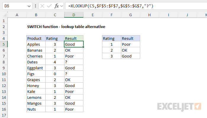
XLOOKUP looks for the rating in C5 in the range F5:F7 and returns the corresponding result from G5:G7. The fourth argument, if_not_found, plays the same role as the default value in SWITCH: it is returned when no match is found. Adding a new rating means adding a row to the table, not editing a formula. Note that XLOOKUP is not required in this case. The VLOOKUP function can do the same job in any version of Excel, with IFERROR to supply the default. If you want a lookup with no table on the worksheet, you can also embed the values in an array constant, as explained in Self-contained VLOOKUP.

SWITCH and performance

You might expect SWITCH to stop evaluating once it finds a matching value, but in fact, Excel evaluates every expression in the formula, including the results for cases that are not used. For most formulas this makes no practical difference. However, when the results in a SWITCH formula involve complex or time-consuming calculations, every one of them runs, even when its value doesn't match, which can degrade performance.

In recursive LAMBDA functions, this behavior can also cause problems, because unused result branches are still evaluated, potentially causing unwanted recursion and a #NUM! error.

If you need "short-circuit" behavior, where Excel stops evaluating after finding the first match, consider using nested IF functions or the CHOOSE function instead. Both IF and CHOOSE perform true short-circuit evaluation, skipping unnecessary calculations once a result has been determined.

SWITCH versus IFS

Like the IFS function, the SWITCH function lets you handle more than one condition in a single self-contained formula, and both functions make it easier to write (and read) a formula with many conditions. The difference is in how the conditions are written. SWITCH compares one expression against a list of values, so the expression appears just once, but SWITCH is limited to exact matching. IFS requires a separate logical test for each condition, so you can use logical operators like greater than (>) and less than (<) as needed. SWITCH also accepts a default value as its last argument, while IFS requires a TRUE test as a workaround. For example, to translate a status code in A1 into a message with a default, the two functions look like this:

=SWITCH(A1,100,"OK",200,"Warning",300,"Error","Invalid")
=IFS(A1=100,"OK",A1=200,"Warning",A1=300,"Error",TRUE,"Invalid")

As a rule of thumb, use SWITCH when you are matching one value against a list of specific values, and use IFS when the conditions involve comparisons or different expressions. You can think of SWITCH as a streamlined version of IFS for situations where one value is matched against a list of possibilities.

SWITCH versus CHOOSE

The CHOOSE function also returns one of several results, but it selects a result by position: an index number of 1 returns the first result, 2 returns the second, and so on. SWITCH selects a result by matching a value, and the values can be anything, including text. The two formulas below return the same result when A1 contains 1, 2, or 3:

=CHOOSE(A1,"Poor","OK","Good") // by position
=SWITCH(A1,1,"Poor",2,"OK",3,"Good") // by value

CHOOSE is the more compact option when the input is already a small sequential number, like the result of the WEEKDAY or MONTH function. SWITCH is the better choice when the values are text, are not sequential, or when a default is needed for unmatched values, since CHOOSE returns #VALUE! for an index number outside its list. CHOOSE does have a performance advantage over SWITCH when either one can be used: it evaluates only the result that is selected, whereas SWITCH evaluates all of them.

Notes

• SWITCH returns the result for the first matching value, so if a value appears more than once, the first pair wins.
• SWITCH performs an exact match only. Matching is not case-sensitive, and wildcards are not supported.
• Text and numbers do not match each other. A code stored as text, like "1", will not match the number 1, and a number will not match a text value.
• To use comparison operators, enter TRUE as the expression and write each value as a logical test, or use the IFS function instead.
• The expression can be a constant, a cell reference, or a formula, and it is evaluated only once.
• Results can be text, numbers, or formulas.
• To set a default result, enter a final argument with no matching value. Without a default, SWITCH returns #N/A when no match is found.
• SWITCH can handle up to 126 value/result pairs.
• SWITCH does not short-circuit; all values and results are evaluated.
• SWITCH is available in Excel 2019 and later. In earlier versions, use a nested IF formula or a lookup function.