Summary
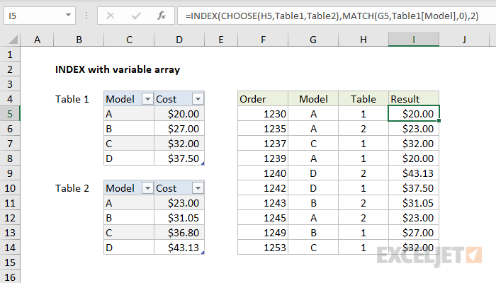
To set up an INDEX and MATCH formula where the array provided to INDEX is variable, you can use the CHOOSE function. In the example shown, the formula in I5, copied down, is:
=INDEX(CHOOSE(H5,Table1,Table2),MATCH(G5,Table1[Model],0),2)
With Table1 and Table2 as indicated in the screenshot.
Generic formula
=INDEX(CHOOSE(number,array1,array2),MATCH(value,range,0))
Explanation
At the core, this is a normal INDEX and MATCH function:
=INDEX(array,MATCH(value,range,0))
Where the MATCH function is used to find the correct row to return from array, and the INDEX function returns the value at that array.
However, in this case we want to make the array variable, so that the range given to INDEX can be changed on the fly. We do this with the CHOOSE function:
CHOOSE(H5,Table1,Table2)
The CHOOSE function returns a value from a list using a given position or index. The value can be a constant, a cell reference, an array, or a range. In the example, the numeric index is provided in column H. When the index number is 1, we use Table1. When the index is 2, we feed Table2 to INDEX:
CHOOSE(1,Table1,Table2) // returns Table1
CHOOSE(2,Table1,Table2) // returns Table2
Note: the ranges provided to CHOOSE don't need to be tables, or named ranges.
In I5, the number in column H is 1, so CHOOSE returns Table1, and the formula resolves to:
=INDEX(Table1,MATCH("A",Table1[Model],0),2)
The MATCH function returns the position of "A" in Table1, which is 1, and INDEX returns the value at row 1, column 2 of Table1, which is $20.00
=INDEX(Table1,1,2) // returns $20.00