Summary
To create an INDEX and MATCH formula that returns a variable number of columns from the source data, you can use the second instance of MATCH to find the numeric index of the desired columns. In the example shown, the formula in cell J5 is:
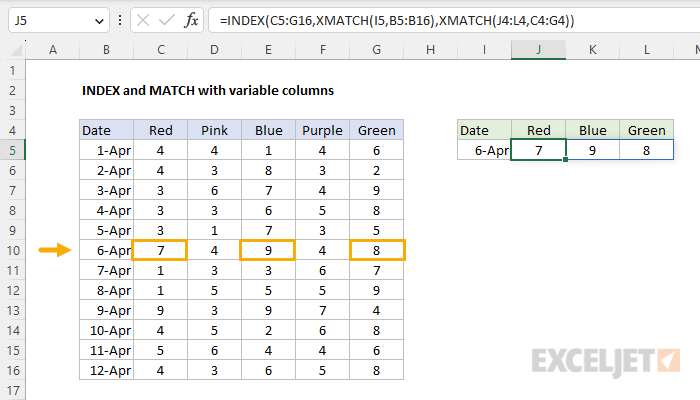
=INDEX(C5:G16,XMATCH(I5,B5:B16),XMATCH(J4:L4,C4:G4))
With "Red", "Blue", and "Green" in the range J4:L4, the formula returns 7, 9, and 8. The values for Red, Green, and Blue on April 6. If the values in J4:L4 are changed to other valid column names, the formula adjusts correspondingly.
Note: See below for a solution based on the XLOOKUP function.
Generic formula
=INDEX(data,XMATCH(A1,array),XMATCH(array,array))
Explanation
In this example, the goal is to demonstrate how an INDEX and (X)MATCH formula can be set up so that the columns returned are variable. This approach illustrates one benefit of the 2-step process used by INDEX and MATCH: Because INDEX expects a numeric index for row and column numbers, it is easy to manipulate these values before they are returned to INDEX. If you are new to INDEX and MATCH, see the overview here How to use INDEX and MATCH.
Two-way INDEX and MATCH
Essentially, this formula employs the two-way INDEX and MATCH approach. The INDEX function is provided with the data to return, and the MATCH function is used twice: once to get the correct row number, and once to get the correct column number(s). The generic syntax looks like this:
=INDEX(data,XMATCH(),XMATCH())
The first MATCH retrieves a row number, and the second MATCH retrieves the column number.
Note: we are using XMATCH in this example because the configuration is slightly easier (XMATCH defaults to exact match), but the original MATCH function will work fine as well.
In the worksheet shown, the specific formula used in cell J5 is as follows:
=INDEX(C5:G16,XMATCH(I5,B5:B16),XMATCH(J4:L4,C4:G4))
Working from the inside out, the first XMATCH function returns a row number:
XMATCH(I5,B5:B16) // returns 6
Because April 6 is the sixth value in the range B5:B16, the first XMATCH function returns 6. The second XMATCH function is used to find the required columns like this:
XMATCH(J4:L4,C4:G4) // returns {1,3,5}
This is the clever bit. Notice the lookup_value is the range J4:L4, which contains "Red", "Blue", and "Green", and the lookup_array is the desired columns in C4:G4. Since we are asking XMATCH to find 3 values, it returns an array with 3 results:
{1,3,5}
The numbers in this array are the numeric positions of the "Red", "Blue", and "Green" in the range C4:G4. After both MATCH formulas run, we have the following inside INDEX:
=INDEX(C5:G16,6,{1,3,5}) // returns {7,9,8}
The INDEX function then returns the values for April 6 (row 6 in the data) for the "Red", "Blue", and "Green" columns only, and the values spill into the range J5:L5.
Note: in a modern version of Excel that supports dynamic array formulas, this formula will just work. In an older version of Excel, you will need to use the MATCH function instead of XMATCH and enter the formula as a multi-cell array formula.
XLOOKUP
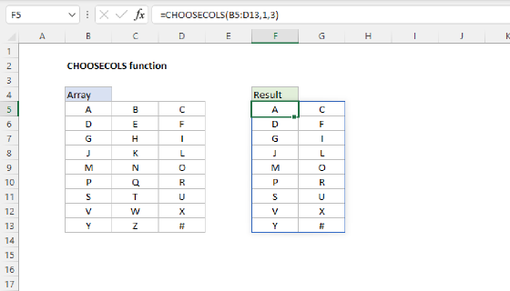
How can this problem be solved using XLOOKUP? One approach is to use the XMATCH function together with the CHOOSECOLS function to alter the original data like this:
=XLOOKUP(I5,B5:B16,CHOOSECOLS(C5:G16,XMATCH(J4:L4,C4:G4)))
Here, the lookup value is the date in cell I5 as before, and the lookup array is the range B5:B16. The return_array is created on the fly with XMATCH and CHOOSECOLS. XMATCH returns the array {1,3,5} as explained above, and the result from MATCH is returned to CHOOSECOLS as the col_num1 argument and C5:G16 as the array. CHOOSECOLS then returns columns 1, 3, and 5 to XLOOKUP as the return_array.
XLOOKUP vs INDEX and MATCH
This problem illustrates a key difference between XLOOKUP and INDEX and MATCH: because INDEX and MATCH formulas use a numeric index for both rows and columns, it is easy to modify these values before they are used in the INDEX function. XLOOKUP on the other hand deals with ranges. To make column ranges dynamic, you sometimes need to use another function like CHOOSECOLS. Both XLOOKUP and INDEX and MATCH offer flexibility and functionality for manipulating and retrieving data, but your choice between them will depend on the specific needs of your project.
For an in-depth comparison, see XLOOKUP vs INDEX and MATCH