Summary
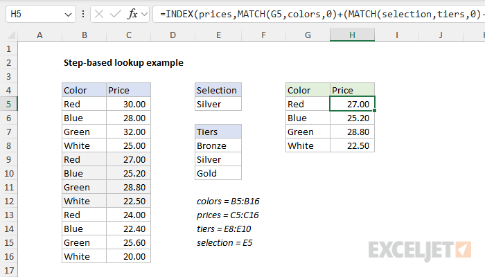
In the worksheet shown, the goal is to look up pricing by tier, but tier is not part of the lookup table. However, because the data follows a predictable pattern, we can use an INDEX and MATCH formula with a numeric "step adjustment" to navigate by tier. In the example shown, the formula in cell H5, copied down, is:
=INDEX(prices,MATCH(G5,colors,0)+(MATCH(selection,tiers,0)-1)*4)
Where prices (C5:C16), colors (B5:B16), selection (E5), and tiers (E8:E10) are named ranges. The result in column H is the correct prices for the four colors based on the tier selected in cell E5. When a different tier is selected, the pricing will update automatically.
You can see an example of this approach applied to a real-world problem here: Income tax bracket calculation.
Explanation
This worksheet demonstrates a clever way to look up prices that change based on a selected tier. Imagine a pricing system where the cost of a product depends on both the product color and a tier (e.g., "Bronze," "Silver," or "Gold"). The challenge is to pull the correct price based on both inputs. At the core of this solution is a standard INDEX and MATCH formula. However, since the prices are organized in blocks corresponding to each tier, we need a way to "step" through the prices correctly based on the selected tier. This is a case where the underlying numeric behavior of INDEX and MATCH formulas lends itself well to simple "step" adjustments based on a clear pattern in the lookup data.
This is a specific technique for doing lookups in a table that is well-structured but not in a way that would make it easy to use a "normal" multiple criteria lookup formula. You can use this approach when the data has a regular pattern that can be navigated numerically. You can see a real-world application of this approach on this page, which explains how to calculate US income tax in brackets based on tax rates published yearly by the IRS. The "step" approach is used to fetch tax rates dynamically based on the selected taxpayer status and year.
Worksheet setup
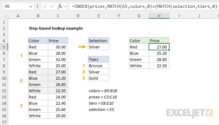
- The worksheet contains pricing for four colors (Red, Blue, Green, and White) in three tiers (Bronze, Silver, and Gold). This means there are 12 prices in total.
- All pricing is stored in columns B and C. The pricing is organized in blocks corresponding to each tier. The order of these blocks follows the order of the tier list in column E.
- Cell E5 contains a dropdown menu for selecting a tier, created with data validation that pulls values from E8:E10. When a user selects a tier in E5, the prices in column H should update to reflect the selected tier.
- For convenience and readability, prices (C5:C16), colors (B5:B16), selection (E5), and tiers (E8:E10) are named ranges.
- The formula in cell H5, copied down, is:
=INDEX(prices,MATCH(G5,colors,0)+(MATCH(selection,tiers,0)-1)*4)
Core INDEX and MATCH formula
The core of this solution is a standard INDEX and MATCH like this:
=INDEX(prices,MATCH(G5,colors,0))
This formula is designed to look up the price for a given color. Inside the INDEX function, the array is given as the named range prices (C5:C16). The row_num is calculated with the MATCH function, which does the work of figuring out the correct row to get a price from:
MATCH(G5,colors,0)
MATCH is configured as follows:
- lookup_value - G5 ("Red")
- lookup_array - colors (B5:B16)
- match_type - 0 (to require an exact match)
Since G5 = "Red", MATCH finds "Red" at row 1 in colors (B5:B16) and returns 1. INDEX then returns 30.00 as a final result:
=INDEX(prices,1) // returns 30.00
In the next row, G6 contains "blue", so MATCH finds "Red" at row 2, and INDEX returns 28.00:
=INDEX(prices,2) // returns 28.00
The same process repeats for "Green" and "White" in the next two rows. This formula works great. However, it has a key limitation: because of how MATCH works, it always retrieves a price for the first match of a color listed in column B. This means the formula only works for Tier 1 pricing (Bronze). To correctly retrieve prices for Silver or Gold (Tier 2 or Tier 3), we need a way to adjust the row number dynamically. This is where the idea of the numeric step adjustment comes into play.
Numeric step adjustment
The second part of the formula is designed to shift the row index as needed to determine the correct price for the selected tier (Bronze, Silver, or Gold):
(MATCH(selection,tiers,0)-1)*4
This is the "numeric step adjustment" part of the formula. Let's break it down logically. This MATCH function locates the selected tier (from E5) in the tiers list (E8:E10) and returns a numeric index. The 0 ensures an exact match. The output from MATCH looks like this:
- If E5 = "Bronze", MATCH returns 1.
- If E5 = "Silver", MATCH returns 2.
- If E5 = "Gold", MATCH returns 3.
The next step is to subtract 1. The logic for this works as follows: Since Bronze is the first tier (starting point), we don’t need to adjust anything when Bronze is selected. However, we do need to adjust the results for Silver and Gold:
- Bronze (Tier 1) → 1 - 1 = 0 → No row shift needed.
- Silver (Tier 2) → 2 - 1 = 1 → We need to shift down one full block.
- Gold (Tier 3) → 3 - 1 = 2 → We need to shift down two full blocks.
The final step is multiplying by 4 to ensure we jump down the correct number of rows.
- Bronze (1st tier): 0 * 4 = 0 → No shift.
- Silver (2nd tier): 1 * 4 = 4 → Move 4 rows down.
- Gold (3rd tier): 2 * 4 = 8 → Move 8 rows down.
By adding this calculated step adjustment, the formula correctly shifts the lookup row to match the selected tier. For example, if G5 = "Red" and E5 = "Silver" the step adjustment works like this:
- MATCH(G5, colors, 0)) returns 1.
- MATCH(selection, tiers, 0) returns 2
- (2 - 1) * 4 = 4, so we move 4 rows down.
- INDEX(prices, 1 + 4) = INDEX(prices, 5)
- The final result is 27.00
To recap, the step adjustment works like this:
- MATCH(selection, tiers, 0) → Finds which tier is selected.
- Subtracting 1 converts to a zero-based index (so Bronze = 0).
- Multiplying by 4 moves the lookup down in full-tier blocks (each containing 4 rows).
- The result is dynamic, so the correct price is pulled for the selected tier.
Conclusion
A step-based lookup formula is a clever way to retrieve data when a table follows a consistent pattern but lacks the information needed to apply multiple criteria. By using a numeric adjustment, this approach allows you to dynamically "jump" to the correct value within a structured table. This method works best when the data follows a regular pattern that can be navigated with predictable steps calculated based on user input. A step-based lookup formula is a simple but powerful way to efficiently look up information without restructuring the data.