Sum lookup values using SUMIF

To sum values retrieved by a lookup operation, you can use SUMPRODUCT with the SUMIF function.

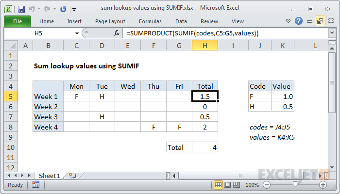
In the example shown, the formula in H5 is:

=SUMPRODUCT(SUMIF(codes,C5:G5,values))

Where codes is the named range J4:J5 and values is the named range K4:K5.

Context

Sometimes you may want to sum multiple values retrieved by a lookup operation. In this example, we want to sum holiday time taken each week based on a code system, where F = a full day, and H = a half day. If a day is blank, no time was taken.

The challenge is to find a formula that both looks up and sums the values associated with F and H.

Explanation

The core of this formula is SUMIF, which is used to lookup the correct values for F and H. Using SUMIF to lookup values is a more advanced technique that works well when the values are numeric, and there are no duplicates in the "lookup table".

The trick in this case is that the criteria for SUMIF is not a single value, but rather an array of values in the range C5:G5:

=SUMPRODUCT(SUMIF(codes,C5:G5,values))

Because we are giving SUMIF more than one criteria, SUMIF will return more than one result. In the example shown, the result of SUMIF is the following array:

{1,0.5,0,0,0}

Note that we correctly get 1 for each "F" and 0.5 for each "H"., and blank values in the week generate zero.

Finally, we use SUMPRODUCT to add up the values in the array returned by SUMIF. Because there is only a single array, SUMPRODUCT simply returns the sum of all values.