Summary
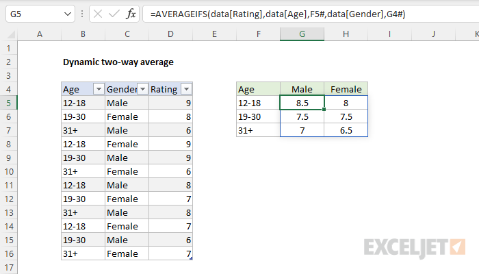
To perform a dynamic two-way average with a formula, you can use an Excel Table, the UNIQUE function, and the AVERAGEIFS function connected to the spill ranges returned by UNIQUE. In the example shown, the formula in cell G5 is:
=AVERAGEIFS(data[Rating],data[Age],F5#,data[Gender],G4#)
Where data is an Excel Table based on the data in B5:D16. The result from AVERAGEIFS spills into the range G5:H7.
Note: Dynamic Array Formulas are only available in Excel 365 and Excel 2021.
Generic formula
=AVERAGEIFS(table[col],table[col],spill1#,table[col],spill2#)
Explanation
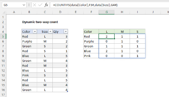
In this example, the goal is to create a formula that performs a dynamic two-way average of all age and gender combinations in the range B5:D16 . The solution shown requires four general steps:
- Create an Excel Table called data
- List unique age groups with UNIQUE function
- List unique genders with UNIQUE function
- Generate all averages in AVERAGEIFS function
Create the Excel Table
One of the key features of an Excel Table is its ability to dynamically resize when rows are added or removed. In this case, all we need to do is create a new table named data with the data shown in B5:D16. You can use the keyboard shortcut Control + T.
Video: How to create an Excel table
The table will now automatically expand or contract as needed.
List unique age groups
The next step is to list the unique age groups in the "Age" column starting in cell F5. For this we use the UNIQUE function. The formula in F5 is:
=UNIQUE(data[Age]) // unique age groups
The result from UNIQUE is a spill range starting in cell F5 listing all of the unique age groups in the Age column of the table. This is what makes this solution fully dynamic. The UNIQUE function will continue to output a list of unique age groups, even as data in the table changes.
Video: Intro to the UNIQUE function
List unique genders
Two perform a two-way average, we also need a list of unique genders starting in cell G4. We can do this with a formula like the one we used for age groups:
UNIQUE(data[Gender]) // unique genders
However, unlike age groups, we need this list to run horizontally across the top of the averages*.* To change the output from vertical to horizontal, we nest the UNIQUE formula in the TRANSPOSE function. The final formula in G4 is:
=TRANSPOSE(UNIQUE(data[Gender])) // horizontal array
The UNIQUE function returns a vertical array like this:
{"Male";"Female"}
And the TRANSPOSE function converts this array into a horizontal array like this:
{"Male","Female"}
Note the comma instead of semicolon in the second array. The UNIQUE function will continue to output a list of unique genders, even if data in the table changes.
Video: What is an array?
Calculate unique averages
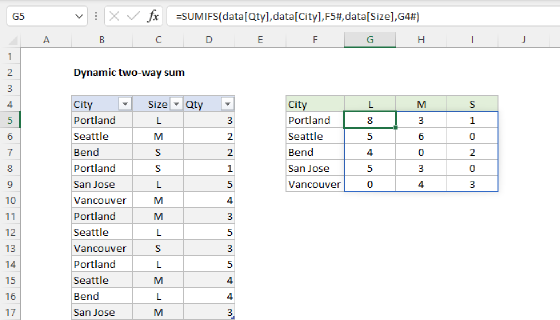
We now have what we need to calculate the averages. Because we have both unique age groups and unique genders on the worksheet as spill ranges, we can use the AVERAGEIFS function for this task. The formula in G5 is:
=AVERAGEIFS(data[Rating],data[Age],F5#,data[Gender],G4#)
The first argument in AVERAGEIFS is average_range. This is the range that contains numbers to average. In this example, this is the Rating column in the table:
data[Rating] // average_range
The other arguments are range/criteria pairs. The first pair targets ages:
data[Age],F5# // all ages, unique ages
The second range/criteria pair targets gender:
data[Gender],G4# // all genders, unique genders
When data changes
The key advantage to this formula approach is that it responds instantly to changes in the data. If new rows are added that refer to existing age groups and genders, the spill ranges returned by AVERAGEIFS remain unchanged, and AVERAGEIFS simply returns an updated set of averages. If new rows are added that include new age groups and/or new genders, these are captured by the UNIQUE function, which expands the spill ranges in F5 and G4 as needed. If rows are deleted from the table, spill ranges contract as needed. In all cases, the spill ranges represent the current list of unique age groups and genders, and the AVERAGEIFS function uses these values to return a current set of averages.
Pivot Table option
A pivot table would also be a good way to solve this problem, and would provide additional capabilities. However, one drawback is that pivot tables need to be refreshed to show the latest data. Formulas, on the other hand, update instantly when data changes.
Dynamic Array Training
If you need training for dynamic arrays in Excel, see our course: Dynamic Array Formulas.