Summary
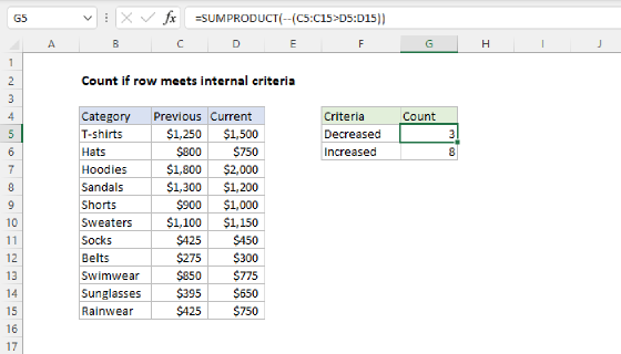
To count rows in a table that meet multiple criteria, without using a helper column, you can use the SUMPRODUCT function. In the example shown, the formula in cell H5 is:
=SUMPRODUCT((E5:E15="tx")*(C5:C15>100)*(MONTH(F5:F15)=3))
The result is 2, since there are two rows where the state is Texas ("TX"), the amount is greater than 100, and the month is March.
Generic formula
=SUMPRODUCT((logical1)*(logical2)*(logical3))
Explanation
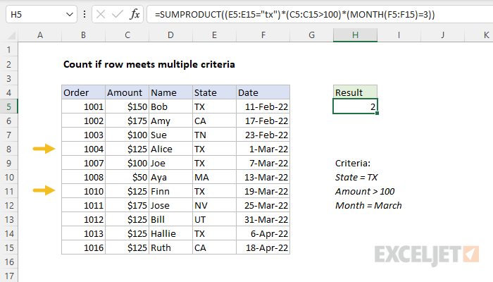
In this example, the goal is to count orders (rows) where the state is Texas ("TX"), the amount is greater than $100, and the month is March. In this case, we can't use COUNTIFS, because COUNTIFS is a range-based function and it won't accept a calculation for a range argument, which we need to determine the month. We could optionally add a helper column that uses the MONTH function to extract the month, then use COUNTIFS, but a better option is to use the SUMPRODUCT function with Boolean logic.
COUNTIFS function
You would think the COUNTIFS function would be the perfect tool for this job, but if we try to use COUNTIFS, we'll run into a problem. The first two conditions are straightforward. We can count orders from Texas ("TX") with amounts greater than $100, like this:
=COUNTIFS(E5:E15,"tx",C5:C15,">100") // returns 4
COUNTIFS returns 4, since there are 4 orders that meet these conditions. However, when we try to extend the criteria to test for orders in March, we run into a problem. The formula below looks fine, but Excel will not let you enter it:
=COUNTIFS(E5:E15,"tx",C5:C15,">100",MONTH(F5:F15),3)
Instead, Excel displays the generic "There's a problem with this formula error" message. This happens because COUNTIFS is a range-based function and it won't accept the array returned by the MONTH function above. The SUMPRODUCT function does not have this limitation and is happy to work with ranges or arrays.
SUMPRODUCT function
The SUMPRODUCT function is programmed to handle array operations natively, without requiring Control + Shift + Enter. Its default behavior is to multiply corresponding elements in one or more arrays together, then sum the products. When given a single array, it returns the sum of the elements in the array. In the example shown, the formula in H5 is:
=SUMPRODUCT((E5:E15="tx")*(C5:C15>100)*(MONTH(F5:F15)=3))
In this example, we are using three logical expressions inside a single array argument, array1. This is typical when using SUMPRODUCT to solve a problem like this because it saves steps and provides full control over the logic used to select data. We could place each expression into a separate argument, but then we would need to coerce logical TRUE and FALSE values to 1s and 0s with another operator like the double negative (--). By placing all expressions into one argument, the math operation of multiplication (*) will automatically convert TRUE and FALSE to 1 and 0.
We have three conditions to apply. The first condition is that the order is from Texas ("TX"):
E5:E15="tx" // state is "tx"
Excel formulas are not case-sensitive, so there is no need to use an uppercase "TX". Because the range E5:E15 contains 11 values, the result is an array that contains 11 TRUE and FALSE values:
{TRUE;FALSE;FALSE;TRUE;TRUE;FALSE;TRUE;FALSE;FALSE;TRUE;FALSE}
The second condition is that the amount is greater than $100:
C5:C15>100 // amount > 100
This expression also returns 11 results:
{TRUE;TRUE;FALSE;TRUE;FALSE;FALSE;TRUE;TRUE;TRUE;TRUE;TRUE}
The third condition is that the month is March. To get the month, we use the MONTH function, which returns a number between 1-12 when given a date:
MONTH(F5:F15)=3 // month is 3
The MONTH function returns an array of 11 month numbers:
={2;2;2;3;3;3;3;3;3;4;4}=3
And the full expression returns this array:
{FALSE;FALSE;FALSE;TRUE;TRUE;TRUE;TRUE;TRUE;TRUE;FALSE;FALSE}
All three arrays are multiplied together because all conditions must be TRUE in order to be included in the final count. In Boolean algebra, multiplication (*) corresponds to AND logic and addition (+) corresponds to OR logic. The math operation automatically converts the TRUE and FALSE values to 1s and 0s. You can visualize the arrays inside of SUMPRODUCT like this:
=SUMPRODUCT({1;0;0;1;1;0;1;0;0;1;0}*{1;1;0;1;0;0;1;1;1;1;1}*{0;0;0;1;1;1;1;1;1;0;0})
After the corresponding values of each array are multiplied together, we have a single array inside the SUMPRODUCT function like this:
=SUMPRODUCT({0;0;0;1;0;0;1;0;0;0;0}) // returns 2
With only one array to process, SUMPRODUCT sums the array and returns 2 as a final result.
Note: The SUMPRODUCT function has been traditionally used to solve problems like this because it has always been able to handle array operations natively, without Control + Shift + Enter. In Excel 365 and Excel 2021, arrays are native and you can use the SUM function instead if you prefer.