Summary
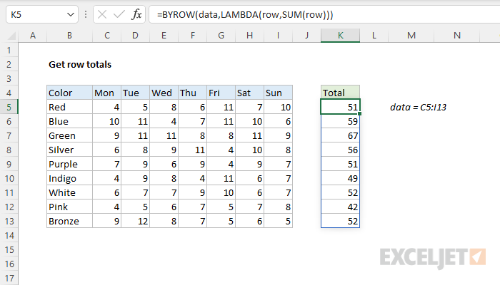
To get an array of row totals based from range of numeric values, you can use a formula based on the BYROW function together with the LAMBDA and SUM functions. In the example shown, the formula in K5 is:
=BYROW(data,LAMBDA(row,SUM(row)))
where data is the named range C5:I13. The result is an array with nine sums, one for each row in the range, as seen in column K.
Note: in older versions of Excel you can use the MMULT function, as explained below.
Generic formula
=BYROW(range,LAMBDA(row,SUM(row)))
Explanation
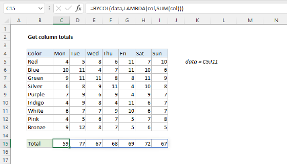
In this example, the goal is to return an array with nine subtotals, one for each of the colors named in column B. The numbers to sum are contained in data which is the named range C5:I13. This is an example of a problem where the goal is to create an array of sums rather than a single sum. We can't use a function like SUM by itself, because SUM will aggregate results and return a single value. In the article below, we look at two approaches, one based on the BYROW function, and one based on the MMULT function.
With the BYROW function
In Excel 365, the most straightforward way to generate subtotals for each row is with the BYROW function. The purpose of BYROW is to process data in a "by row" fashion. For example, if BYROW is given an array with 10 rows, BYROW will return single array with 10 results. In the example shown, the formula in K5 is:
=BYROW(data,LAMBDA(row,SUM(row)))
The calculation performed on each row is provided by a custom LAMBDA function, which must return a single result for each row. In this example, the LAMBDA function used in BYROW sums each row like this:
LAMBDA(row,SUM(row)) // sum each row
The result is an array of sums, one per row, that spill into the range K5:K13. This result is fully dynamic. If data values change, or if the data range expands or contracts, the output from BYROW will update as needed. Although this example deals with totals, the same pattern can be used to calculate other information about rows, including max, min, average, etc. like this:
=BYROW(data,LAMBDA(row,MAX(row))) // max
=BYROW(data,LAMBDA(row,MIN(row))) // min
=BYROW(data,LAMBDA(row,AVERAGE(row))) // average
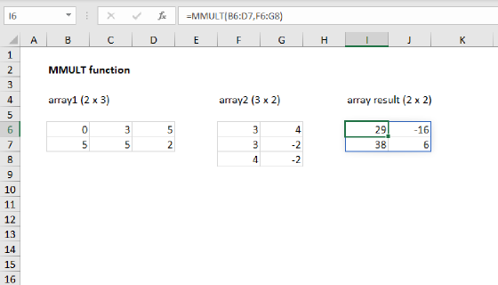
With the MMULT function
Another way to solve this problem is with the MMULT function, which performs matrix multiplication. MMULT takes two arrays, array1 and array2, and requires that the number of columns in array1 be the same as the number of rows in array2. The resulting matrix will have same number of rows as the first matrix, and the same number of columns as the second matrix. The MMULT formula looks like this:
=MMULT(--data,TRANSPOSE(COLUMN(data)^0))
The first array is simply all values in data, the named range C5:I13:
=MMULT(--data
To protect against blank cells, which will cause MMULT to throw #VALUE! error, we use a double negative (--) to force any empty cells to zero.
Next, we need to create array2. The first array contains 7 columns, so we need the second array to contain 7 rows. We want just a single column of results, so the second array should be 7 rows by 1 column (7 x 1). Also, because we don't want to change any values, the array should contain only the number 1 (i.e. multiplying by 1 does not change the original value). Array2 is generated with the TRANSPOSE function and the COLUMN function like this:
TRANSPOSE(COLUMN(data)^0)
While slightly cryptic, this syntax above is a clever way to accomplish the task. The COLUMN function returns a 1 x 7 array of column numbers:
COLUMN(data) // returns {3,4,5,6,7,8,9}
Next, these numbers are raised to the power of zero with exponent operator (^), which creates a 1 x 7 array of 1s:
COLUMN(data)^0) // returns {1,1,1,1,1,1,1}
And the TRANSPOSE function flips the array from 1 x 7 to 7 x 1:
TRANSPOSE({1,1,1,1,1,1,1}) // returns {1;1;1;1;1;1;1}
The result is handed off to the MMULT function as array2. The MMULT function then performs matrix multiplication with the two arrays, and returns a subtotal for each row:
=MMULT(--data,{1;1;1;1;1;1;1})
returns the array:
{51;59;67;56;51;49;52;42;52}
These values are returned to cell K5, and spill into the range K5:K13.
SEQUENCE alternative
Another way to construct array2 inside MMULT is with the SEQUENCE function like this:
=MMULT(--data,SEQUENCE(COLUMNS(data),1,1,0))
This formula works the same way, but array2 is created with the SEQUENCE function directly:
SEQUENCE(COLUMNS(data),1,1,0) // returns {1;1;1;1;1;1;1}
Note we use the COLUMNS function to tell SEQUENCE how many rows to create (7).