Row is blank

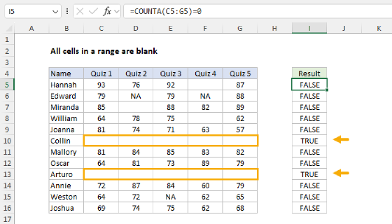
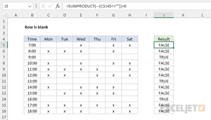
To determine if all cells in a row are blank (i.e. empty), you can use a formula based on the SUMPRODUCT function. In the example shown, the formula in cell J5 is:

=SUMPRODUCT(--(C5:H5<>""))=0

As the formula is copied down, it returns TRUE if all cells in a row are empty and FALSE if any cell contains a value. In newer versions of Excel, you can also use the BYROW function, as explained below.

Explanation

The goal is to use a formula to check if all cells in a row are blank or empty and return TRUE or FALSE. One way to solve this problem is with the SUMPRODUCT function, as seen in the worksheet above. Another approach is to use the newer BYROW function. Both methods are described below.

SUMPRODUCT function

The SUMPRODUCT function is a Swiss Army Knife function that appears in all kinds of formulas because it can handle many array operations natively in older versions of Excel. In this case, the formula we are using in cell J5 is:

=SUMPRODUCT(--(C5:H5<>""))=0

Working from the inside out, the expression below is used to check for data in row 5 like this:

C5:H5<>""

The <> operator means "not equal to" so <>"" means "not empty". Notice we are excluding column B which contains times. Because there are six cells in the range C5:H5, the expression returns six results in an array like this:

=SUMPRODUCT(--({FALSE,FALSE,TRUE,FALSE,TRUE,TRUE}))=0

In this array, FALSE corresponds to cells that are not empty and TRUE corresponds to cells that are empty. Next, we use a double negative (--) operation to convert TRUE values to 1 and FALSE values to 0. The result looks like this:

=SUMPRODUCT({0,0,1,0,1,1})=0

SUMPRODUCT then sums the values in the array and returns 3:

=3=0 // returns FALSE

The final result in J5 is FALSE since 3 is not equal to zero. This formula will return TRUE only when all cells in a given row are empty. For example, in row 7 which is empty, the formula evaluates like this:

=SUMPRODUCT(--(C7:H7<>""))=0
=SUMPRODUCT(--({FALSE,FALSE,FALSE,FALSE,FALSE,FALSE}))=0
=SUMPRODUCT({0,0,0,0,0,0})=0
=TRUE

See Boolean operations in array formulas for more information about the logic used in SUMPRODUCT.

BYROW function

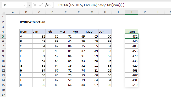
In newer versions of Excel, you can use the BYROW function to test all rows in a range in one step. The purpose of BYROW is to process data in an array or range in a "by row" fashion. BYROW applies a custom LAMBDA function to each row in a range or array and returns one result per row as a single array. You can see the result in the worksheet below:

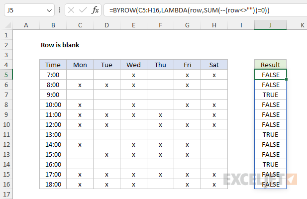
Testing for blank rows with the BYROW function

The formula used in cell J5 is:

=BYROW(C5:H16,LAMBDA(row,SUM(--(row<>""))=0))

The BYROW function delivers the range C5:H16 one row at a time to the LAMBDA function, which uses the SUM function and the same Boolean logic explained above to count non-blank cells. The result from SUM is then compared to zero to force a TRUE or FALSE result. After processing the entire range, BYROW delivers all results in a single array:

{FALSE;FALSE;TRUE;FALSE;FALSE;FALSE;TRUE;FALSE;FALSE;TRUE;FALSE;FALSE}

Notice the array contains 12 results because the original range contains 12 rows. These results spill into the range J5:J16. Other than convenience, the advantage of using BYROW like this is that the results can be used in other functions. For example, you can use BYROW inside the FILTER function to remove blank rows.