Summary
To assign rank without ties, you can use a formula based on the RANK and COUNTIF functions. In the example shown, the formula in E5 is:
=RANK(C5,points)+COUNTIF($C$5:C5,C5)-1
where "points" is a named range.
Generic formula
=RANK(A1,range)+COUNTIF(exp_range,A1)-1
Explanation
This formula breaks ties with a simple approach: this first tie in a list "wins" and is assigned the higher rank. The first part of the formula uses the RANK function normally:
=RANK(C5,points)
Rank returns a computed rank, which will include ties when the values being ranked include duplicates. Note that the RANK function by itself will assign the same rank to duplicate values, and skip the next rank value. You can see this in the Rank 1 column, rows 8 and 9 in the worksheet.
The second part of the formula breaks the tie with COUNTIF:
COUNTIF($C$5:C5,C5)-1
Note the range we give COUNTIF is an expanding reference: the first reference is absolute and the second is relative. As long as a value appears just once, this expression cancels itself out – COUNTIF returns 1, from which 1 is subtracted.
However, when a duplicate number is encountered, COUNTIF returns 2, the expression returns 1, and the rank value is increased by 1. Essentially, this "replaces" the rank value that was skipped originally.
The same process repeats as the formula is copied down the column. If another duplicate is encountered, the rank value is increased by 2, and so on.