Summary
To break ties, you can use a helper column and the COUNTIF function to adjust values so that they don't contain duplicates, and therefore won't result in ties. In the example shown, the formula in D5 is:
=C5+(COUNTIF($C$5:C5,C5)-1)*0.01
Note: in Excel 2021 and later, a better approach to this kind of problem is to use the FILTER function as explained here.
Generic formula
=A1+(COUNTIF(exp_rng,A1)-1)*adjustment
Explanation
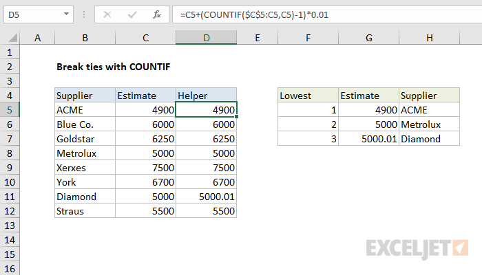
In this example, the goal is to retrieve information about the lowest three estimates in the data shown. The problem is that there are some duplicate values in the estimate column. This means we will have some trouble trying to display the names of the 2nd and 3rd lowest suppliers because the tie values will cause INDEX to return the same name. One way to break ties like this is to add a helper column with values that have been adjusted, and then rank those values instead of the originals. In this example, the logic used to adjust values is random - the first duplicate value will "win", but you can adjust the formula to use logic that fits your particular situation and use case.
COUNTIF with expanding reference
At the core, this formula uses the COUNTIF function and an expanding range to count occurrences of values. The expanding reference is used so that COUNTIFS returns a running count of occurrences, instead of a total count for each value:
COUNTIF($C$5:C5,C5)
Next, 1 is subtracted from the result (which makes the count of all non-duplicate values zero) and the result is multiplied by 0.01. This value is the "adjustment", and is intentionally small so as not to materially impact the original value.
In the example shown, Metrolux and Diamond both have the same estimate of $5000. Since Metrolux appears first in the list, the running count of 5000 is 1 and is canceled out by subtracting 1, so the estimate remains unchanged in the helper column:
=C8+(COUNTIF($C$5:C8,C8)-1)*0.01
=C8+(1-1)*0.01
=C8+0
=C8
However, for Diamond, the running count of 5000 is 2, so the estimate is adjusted:
=C11+(COUNTIF($C$5:C11,C11)-1)*0.01
=C11+(2-1)*0.01
=C11+1*0.01
=C11+0.01
Finally, the adjusted values are used for ranking instead of the original values in columns G and H. The formula in G5 is:
=SMALL($D$5:$D$12,F5)
The formula in H5:
=INDEX($B$5:$B$12,MATCH(G5,$D$5:$D$12,0))
For a detailed explanation of these formulas, see this example.
Temporary helper column
If you don't want to use a helper column in the final solution, you can use a helper column temporarily to get calculated values, then use Paste Special to convert values "in place" and delete the helper column afterward. This video demonstrates the technique.