Summary
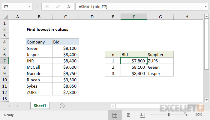
To find the n lowest values in a set of data, you can use the SMALL function. This can be combined with INDEX as shown below to retrieve associated values. In the example shown, the formula in F7 is:
=SMALL(bid,E7)
Note: this worksheet has two named ranges: bid (C5:C12), and company (B5:B12), used for convenience and readability only.
Generic formula
=SMALL(range,n)
Explanation
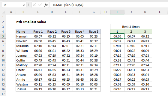
The SMALL function retrieves the smallest values from data based on a given rank. For example:
=SMALL(range,1) // smallest
=SMALL(range,2) // 2nd smallest
=SMALL(range,3) // 3rd smallest
In the worksheet shown, the rank (which is provided to SMALL as the k argument) comes from numbers in column E.
Retrieve associated values
To retrieve the name of the company associated with the smallest bids, we can use an INDEX and MATCH formula. In the worksheet shown, the formula in G7 is:
=INDEX(company,MATCH(F7,bid,0))
Here, the value in column F is used as the lookup value inside MATCH, with the named range bid (C5:C12) for lookup_array, and match_type set to zero to force an exact match. MATCH returns the location of the value to INDEX as the row number. INDEX then retrieves the corresponding value from the named range company (B5:B12). An all-in-one formula to get the company name in one step would look like this:
=INDEX(company,MATCH(SMALL(bid,E7),bid,0))
Note: if your values contain duplicates you may get ties when you try to rank. You can use a formula like this to break times.
FILTER option
The FILTER function provides a better way to retrieve the top or bottom n values from a set of data. See this page for an example.